
1910/1914
This is a restored edition of Calculus Made Easy: the author's own words, unchanged. Every plate carries a caption and alt text written for this edition, beginning with the label the book printed. The original is available from Project Gutenberg. Also available as an epub. More restored editions.
Silvanus P. Thompson (1851–1916) was a physicist and an electrical engineer, and for more than thirty years the principal of the Finsbury Technical College in London, where he taught the young engineers who were building the telephone exchanges, power stations and electric tramways of the time. He was a Fellow of the Royal Society, he wrote the standard textbooks on electricity and on the dynamo, and he gave the Royal Institution Christmas Lectures of 1896, which this collection publishes as Light Visible and Invisible.
Calculus Made Easy came out in 1910 with no author's name on it. The title page said only "By F.R.S.", and the motto on the back of it, "What one fool can do, another can", was credited to an Ancient Simian Proverb. Thompson thought the difficulty of the calculus was mostly a matter of how it was taught: the textbooks were written by "clever fools" who wanted to show how clever they were. So he explains the two dreadful symbols first, and then does everything else with small quantities that grow, slopes of curves, and a great deal of arithmetic worked out in full. This is the second edition of 1914, enlarged with more worked examples and exercises.
A few conventions are worth knowing. Thompson writes the base of natural logarithms as ε, epsilon, where most books now write e. His "differential coefficient" is what is now usually called the derivative. Money is in pounds, shillings and pence. His page references ("see p. 76") are to the 1914 printing and are kept as he wrote them.
This is a restored edition: Thompson's words are unchanged. The Project Gutenberg transcription it is built from sets every formula, more than three thousand six hundred of them, as a separate picture. This edition typesets them as mathematics, so they reflow and can be read aloud, and it adds a description and alt text for each of the sixty-six figures. Gutenberg's transcribers corrected a number of misprints and recomputed several tables of figures in Chapter XIV, and those corrections are kept. Three pairs of figures, 12 and 13, 38 and 39, and 44 and 45, carried each other's numbers in the transcription and are numbered here as Thompson's text describes them. Two words the transcription had modernised are restored as printed: "one billionth", in the British sense of a million millionths, and Sandy's "bang went saxpence". The edition also adds modern typesetting, a proper ebook, and this introduction.
Chapter I: To Deliver You from the Preliminary Terrors
Chapter II: On Different Degrees of Smallness
Chapter III: On Relative Growings
Note to Chapter III: How to Read Differentials
Chapter V: Next Stage. What to Do with Constants
Chapter VI: Sums, Differences, Products and Quotients
Chapter VII: Successive Differentiation
Chapter VIII: When Time Varies
Chapter IX: Introducing a Useful Dodge
Chapter X: Geometrical Meaning of Differentiation
Chapter XII: Curvature of Curves
Chapter XIII: Other Useful Dodges
Chapter XIV: On True Compound Interest and the Law of Organic Growth
Chapter XV: How to Deal with Sines and Cosines
Chapter XVI: Partial Differentiation
Chapter XVIII: Integrating as the Reverse of Differentiating
Chapter XIX: On Finding Areas by Integrating
Chapter XX: Dodges, Pitfalls, and Triumphs
Chapter XXI: Finding Some Solutions
	What one fool can do, another can.
	(Ancient Simian Proverb.)
The surprising success of this work has led the author to add a considerable number of worked examples and exercises. Advantage has also been taken to enlarge certain parts where experience showed that further explanations would be useful.
The author acknowledges with gratitude many valuable suggestions and letters received from teachers, students, and-critics.
October, 1914.
CONSIDERING how many fools can calculate, it is surprising that it should be thought either a difficult or a tedious task for any other fool to learn how to master the same tricks.
Some calculus-tricks are quite easy. Some are enormously difficult. The fools who write the textbooks of advanced mathematics—and they are mostly clever fools-seldom take the trouble to show you how easy the easy calculations are. On the contrary, they seem to desire to impress you with their tremendous cleverness by going about it in the most difficult way.
Being myself a remarkably stupid fellow, I have had to unteach myself the difficulties, and now beg to present to my fellow fools the parts that are not hard. Master these thoroughly, and the rest will follow. What one fool can do, another can.
THE preliminary terror, which chokes off most fifth-form boys from even attempting to learn how to calculate, can be abolished once for all by simply stating what is the meaning-in common-sense terms-of the two principal symbols that are used in calculating.
These dreadful symbols are:
(1) which merely means "a little bit of."
Thus means a little bit of ; or means a little bit of . Ordinary mathematicians think it more polite to say "an element of," instead of "a little bit of." Just as you please. But you will find that these little bits (or elements) may be considered to be indefinitely small.
(2) which is merely a long , and may be called (if you like) "the sum of."
Thus means the sum of all the little bits of ; or means the sum of all the little bits of . Ordinary mathematicians call this symbol "the integral of." Now any fool can see that if is considered as made up of a lot of little bits, each of which is called , if you add them all up together you get the sum of all the 's, (which is the same thing as the whole of ). The word "integral" simply means "the whole." If you think of the duration of time for one hour, you may (if you like) think of it as cut up into 3600 little bits called seconds. The whole of the 3600 little bits added up together make one hour.
When you see an expression that begins with this terrifying symbol, you will henceforth know that it is put there merely to give you instructions that you are now to perform the operation (if you can) of totalling up all the little bits that are indicated by the symbols that follow.
That's all.
WE shall find that in our processes of calculation we have to deal with small quantities of various degrees of smallness.
We shall have also to learn under what circumstances we may consider small quantities to be so minute that we may omit them from consideration. Everything depends upon relative minuteness.
Before we fix any rules let us think of some familiar cases. There are 60 minutes in the hour, 24 hours in the day, 7 days in the week. There are therefore 1440 minutes in the day and 10080 minutes in the week.
Obviously 1 minute is a very small quantity of time compared with a whole week. Indeed, our forefathers considered it small as compared with an hour, and called it "one minùte," meaning a minute fraction —namely one sixtieth—of an hour. When they came to require still smaller subdivisions of time, they divided each minute into 60 still smaller parts, which, in Queen Elizabeth's days, they called "second minùtes" (i.e. small quantities of the second order of minuteness). Nowadays we call these small quantities of the second order of smallness "seconds." But few people know why they are so called.
Now if one minute is so small as compared with a whole day, how much smaller by comparison is one second!
Again, think of a farthing as compared with a sovereign: it is barely worth more than part. A farthing more or less is of precious little importance compared with a sovereign: it may certainly be regarded as a small quantity. But compare a farthing with : relatively to this greater sum, the farthing is of no more importance than of a farthing would be to a sovereign. Even a golden sovereign is relatively a negligible quantity in the wealth of a millionaire.
Now if we fix upon any numerical fraction as constituting the proportion which for any purpose we call relatively small, we can easily state other fractions of a higher degree of smallness. Thus if, for the purpose of time, be called a small fraction, then of (being a small fraction of a small fraction) may be regarded as a small quantity of the second order of smallness.
Footnote: The mathematicians talk about the second order of "magnitude" (i.e. greatness) when they really mean second order of smallness. This is very confusing to beginners.
Or, if for any purpose we were to take 1 per cent. as a small fraction, then 1 per cent. of 1 per cent. would be a small fraction of the second order of smallness; and would be a small fraction of the third order of smallness, being 1 per cent. of 1 per cent. of 1 per cent.
Lastly, suppose that for some very precise purpose we should regard as "small." Thus, if a first-rate chronometer is not to lose or gain more than half a minute in a year, it must keep time with an accuracy of 1 part in . Now if, for such a purpose, we regard (or one millionth) as a small quantity, then of , that is (or one billionth) will be a small quantity of the second order of smallness, and may be utterly disregarded, by comparison.
Then we see that the smaller a small quantity itself is, the more negligible does the corresponding small quantity of the second order become. Hence we know that in all cases we are justified in neglecting the small quantities of the second-or third (or higher)—orders, if only we take the small quantity of the first order small enough in itself.
But, it must be remembered, that small quantities if they occur in our expressions as factors multiplied by some other factor, may become important if the other factor is itself large. Even a farthing becomes important if only it is multiplied by a few hundred.
Now in the calculus we write for a little bit of . These things such as , and , and , are called "differentials," the differential of , or of , or of , as the case may be. [You read them as dee-eks, or dee-you, or dee-wy.] If be a small bit of , and relatively small of itself, it does not follow that such quantities as , or , or are negligible. But would be negligible, being a small quantity of the second order.
A very simple example will serve as illustration.
Let us think of as a quantity that can grow by a small amount so as to become , where is the small increment added by growth. The square of this is . The second term is not negligible because it is a first-order quantity; while the third term is of the second order of smallness, being a bit of, a bit of . Thus if we took to mean numerically, say, of , then the second term would be of , whereas the third term would be of . This last term is clearly less important than the second. But if we go further and take to mean only of , then the second term will be of , while the third term will be only of .
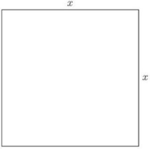
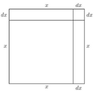
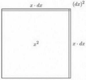
Geometrically this may be depicted as follows: Draw a square (Fig. 1) the side of which we will take to represent . Now suppose the square to grow by having a bit added to its size each way. The enlarged square is made up of the original square , the two rectangles at the top and on the right, each of which is of area (or together ), and the little square at the top right-hand corner which is . In Fig. 2 we have taken as quite a big fraction of —about . But suppose we had taken it only —about the thickness of an inked line drawn with a fine pen. Then the little corner square will have an area of only of , and be practically invisible. Clearly is negligible if only we consider the increment to be itself small enough.
Let us consider a simile.
Suppose a millionaire were to say to his secretary: next week I will give you a small fraction of any money that comes in to me. Suppose that the secretary were to say to his boy: I will give you a small fraction of what I get. Suppose the fraction in each case to be part. Now if Mr. Millionaire received during the next week , the secretary would receive and the boy 2 shillings. Ten pounds would be a small quantity compared with ; but two shillings is a small small quantity indeed, of a very secondary order. But what would be the disproportion if the fraction, instead of being , had been settled at part? Then, while Mr. Millionaire got his , Mr. Secretary would get only , and the boy less than one farthing!
The witty Dean Swift once wrote:
Footnote: On Poetry: a Rhapsody (p. 20), printed 1733—usually misquoted.
	"So, Nat'ralists observe, a Flea
	"Hath smaller Fleas that on him prey.
	"And these have smaller Fleas to bite 'em,
	"And so proceed ad infinitum."
An ox might worry about a flea of ordinary size—a small creature of the first order of smallness. But he would probably not trouble himself about a flea's flea; being of the second order of smallness, it would be negligible. Even a gross of fleas' fleas would not be of much account to the ox.
ALL through the calculus we are dealing with quantities that are growing, and with rates of growth. We classify all quantities into two classes: constants and variables. Those which we regard as of fixed value, and call constants, we generally denote algebraically by letters from the beginning of the alphabet, such as , , or ; while those which we consider as capable of growing, or (as mathematicians say) of "varying," we denote by letters from the end of the alphabet, such as , or sometimes .
Moreover, we are usually dealing with more than one variable at once, and thinking of the way in which one variable depends on the other: for instance, we think of the way in which the height reached by a projectile depends on the time of attaining that height. Or we are asked to consider a rectangle of given area, and to enquire how any increase in the length of it will compel a corresponding decrease in the breadth of it. Or we think of the way in which any variation in the slope of a ladder will cause the height that it reaches, to vary.
Suppose we have got two such variables that depend one on the other. An alteration in one will bring about an alteration in the other, because of this dependence. Let us call one of the variables , and the other that depends on it .
Suppose we make to vary, that is to say, we either alter it or imagine it to be altered, by adding to it a bit which we call . We are thus causing to become . Then, because has been altered, will have altered also, and will have become . Here the bit may be in some cases positive, in others negative; and it won't (except by a miracle) be the same size as .
Take two examples.
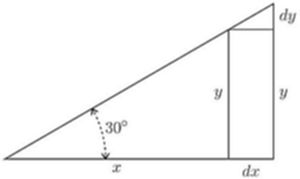
(1) Let and be respectively the base and the height of a right-angled triangle (Fig. 4), of which the slope of the other side is fixed at . If we suppose this triangle to expand and yet keep its angles the same as at first, then, when the base grows so as to become , the height becomes . Here, increasing results in an increase of . The little triangle, the height of which is , and the base of which is , is similar to the original triangle; and it is obvious that the value of the ratio is the same as that of the ratio . As the angle is it will be seen that here
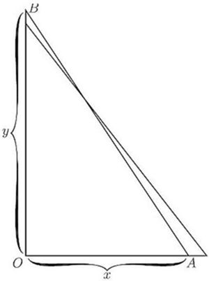
(2) Let represent, in Fig. 5, the horizontal distance, from a wall, of the bottom end of a ladder, , of fixed length; and let be the height it reaches up the wall. Now clearly depends on . It is easy to see that, if we pull the bottom end a bit further from the wall, the top end will come down a little lower. Let us state this in scientific language. If we increase to , then will become ; that is, when receives a positive increment, the increment which results to is negative.
Yes, but how much? Suppose the ladder was so long that when the bottom end was 19 inches from the wall the top end reached just 15 feet from the ground. Now, if you were to pull the bottom end out 1 inch more, how much would the top end come down? Put it all into inches: inches, inches. Now the increment of which we call , is 1 inch: or inches.
How much will be diminished? The new height will be . If we work out the height by Euclid I. 47, then we shall be able to find how much will be. The length of the ladder is
Clearly then, the new height, which is , will be such that Now is 180, so that is inch.
So we see that making an increase of 1 inch has resulted in making a decrease of 0.11 inch.
And the ratio of to may be stated thus:
It is also easy to see that (except in one particular position) will be of a different size from .
Now right through the differential calculus we are hunting, hunting, hunting for a curious thing, a mere ratio, namely, the proportion which bears to when both of them are indefinitely small.
It should be noted here that we can only find this ratio when and are related to each other in some way, so that whenever varies does vary also. For instance, in the first example just taken, if the base of the triangle be made longer, the height of the triangle becomes greater also, and in the second example, if the distance of the foot of the ladder from the wall be made to increase, the height reached by the ladder decreases in a corresponding manner, slowly at first, but more and more rapidly as becomes greater. In these cases the relation between and is perfectly definite, it can be expressed mathematically, being and (where is the length of the ladder) respectively, and has the meaning we found in each case.
If, while is, as before, the distance of the foot of the ladder from the wall, is, instead of the height reached, the horizontal length of the wall, or the number of bricks in it, or the number of years since it was built, any change in would naturally cause no change whatever in ; in this case has no meaning whatever, and it is not possible to find an expression for it. Whenever we use differentials , , , etc., the existence of some kind of relation between , etc., is implied, and this relation is called a "function" in , etc.; the two expressions given above, for instance, namely and , are functions of and . Such expressions contain implicitly (that is, contain without distinctly showing it) the means of expressing either in terms of or in terms of , and for this reason they are called implicit functions in and ; they can be respectively put into the forms
These last expressions state explicitly (that is, distinctly) the value of in terms of , or of in terms of , and they are for this reason called explicit functions of or . For example is an implicit function in and ; it may be written (explicit function of ) or (explicit function of ). We see that an explicit function in , , , etc., is simply something the value of which changes when , , , etc., are changing, either one at the time or several together. Because of this, the value of the explicit function is called the dependent variable, as it depends on the value of the other variable quantities in the function; these other variables are called the independent variables because their value is not determined from the value assumed by the function. For example, if , and are the independent variables, and is the dependent variable.
Sometimes the exact relation between several quantities , , either is not known or it is not convenient to state it; it is only known, or convenient to state, that there is some sort of relation between these variables, so that one cannot alter either or or singly without affecting the other quantities; the existence of a function in , , is then indicated by the notation (implicit function) or by , or (explicit function). Sometimes the letter or is used instead of , so that , and all mean the same thing, namely, that the value of depends on the value of in some way which is not stated.
We call the ratio "the differential coefficient of with respect to ." It is a solemn scientific name for this very simple thing. But we are not going to be frightened by solemn names, when the things themselves are so easy. Instead of being frightened we will simply pronounce a brief curse on the stupidity of giving long crack-jaw names; and, having relieved our minds, will go on to the simple thing itself, namely the ratio .
In ordinary algebra which you learned at school, you were always hunting after some unknown quantity which you called or ; or sometimes there were two unknown quantities to be hunted for simultaneously. You have now to learn to go hunting in a new way; the fox being now neither nor . Instead of this you have to hunt for this curious cub called . The process of finding the value of is called "differentiating." But, remember, what is wanted is the value of this ratio when both and are themselves indefinitely small. The true value of the differential coefficient is that to which it approximates in the limiting case when each of them is considered as infinitesimally minute.
Let us now learn how to go in quest of .
It will never do to fall into the schoolboy error of thinking that means times , for is not a factor-it means "an element of" or "a bit of" whatever follows. One reads thus: "dee-eks."
In case the reader has no one to guide him in such matters it may here be simply said that one reads differential coefficients in the following way. The differential coefficient
So also is read "dee-you by dee-tee." Second differential coefficients will be met with later on. They are like this: and it means that the operation of differentiating with respect to has been (or has to be) performed twice over.
Another way of indicating that a function has been differentiated is by putting an accent to the symbol of the function. Thus if , which means that is some unspecified function of (see p. 13), we may write instead of . Similarly, will mean that the original function has been differentiated twice over with respect to .
NOW let us see how, on first principles, we can differentiate some simple algebraical expression.
Let us begin with the simple expression . Now remember that the fundamental notion about the calculus is the idea of growing. Mathematicians call it varying. Now as and are equal to one another, it is clear that if grows, will also grow. And if grows, then will also grow. What we have got to find out is the proportion between the growing of and the growing of . In other words our task is to find out the ratio between and , or, in brief, to find the value of .
Let , then, grow a little bit bigger and become ; similarly, will grow a bit bigger and will become . Then, clearly, it will still be true that the enlarged will be equal to the square of the enlarged . Writing this down, we have:
Doing the squaring we get:
What does mean? Remember that meant a bit-a little bit-of . Then will mean a little bit of a little bit of ; that is, as explained above (p. 4), it is a small quantity of the second order of smallness. It may therefore be discarded as quite inconsiderable in comparison with the other terms. Leaving it out, we then have:
Now ; so let us subtract this from the equation and we have left
Dividing across by , we find
Now this is what we set out to find. The ratio of the growing of to the growing of is, in the case before us, found to be .
Footnote: N.B.—This ratio is the result of differentiating with respect to . Differentiating means finding the differential coefficient. Suppose we had some other function of , as, for example, . Then if we were told to differentiate this with respect to , we should have to find , or, what is the same thing, . On the other hand, we may have a case in which time was the independent variable (see p. 14), such as this: . Then, if we were told to differentiate it, that means we must find its differential coefficient with respect to . So that then our business would be to try to find , that is, to find .
Suppose and . Then let grow till it becomes 101 (that is, let ). Then the enlarged will be 10,201. But if we agree that we may ignore small quantities of the second order, 1 may be rejected as compared with 10,000; so we may round off the enlarged to 10,200. has grown from 10,000 to 10,200; the bit added on is , which is therefore 200.
. According to the algebra-working of the previous paragraph, we find . And so it is; for and .
But, you will say, we neglected a whole unit.
Well, try again, making a still smaller bit.
Try . Then , and
Now the last figure 1 is only one-millionth part of the 10,000, and is utterly negligible; so we may take 10,020 without the little decimal at the end.
And this makes ; and , which is still the same as .
Try differentiating in the same way.
We let grow to , while grows to .
Then we have
Doing the cubing we obtain
Now we know that we may neglect small quantities of the second and third orders; since, when and are both made indefinitely small, and will become indefinitely smaller by comparison. So, regarding them as negligible, we have left:
But ; and, subtracting this, we have:
Try differentiating . Starting as before by letting both and grow a bit, we have:
Working out the raising to the fourth power, we get
Then striking out the terms containing all the higher powers of , as being negligible by comparison, we have
Subtracting the original , we have left
Now all these cases are quite easy. Let us collect the results to see if we can infer any general rule. Put them in two columns, the values of in one and the corresponding values found for in the other: thus
| y | |
Just look at these results: the operation of differentiating appears to have had the effect of diminishing the power of by 1 (for example in the last case reducing to ), and at the same time multiplying by a number (the same number in fact which originally appeared as the power). Now, when you have once seen this, you might easily conjecture how the others will run. You would expect that differentiating would give , or differentiating would give . If you hesitate, try one of these, and see whether the conjecture comes right.
Try .
Then
Neglecting all the terms containing small quantities of the higher orders, we have left
Following out logically our observation, we should conclude that if we want to deal with any higher power,—call it —we could tackle it in the same way.
Let ,
then we should expect to find that
For example, let , then ; and differentiating it would give .
And, indeed, the rule that differentiating gives as the result is true for all cases where is a whole number and positive. [Expanding by the binomial theorem will at once show this.] But the question whether it is true for cases where has negative or fractional values requires further consideration.
Case of a negative power
Let . Then proceed as before:
Expanding this by the binomial theorem (see p. 137), we get
So, neglecting the small quantities of higher orders of smallness, we have: Subtracting the original , we find And this is still in accordance with the rule inferred above.
Case of a fractional power
Let . Then, as before,
Subtracting the original , and neglecting higher powers we have left: and . Agreeing with the general rule.
Summary. Let us see how far we have got. We have arrived at the following rule: To differentiate , multiply by the power and reduce the power by one, so giving us as the result.
Exercises I. (See p. 252 for Answers.)
Differentiate the following:
(1)
(2)
(3)
(4)
(5)
(6)
(7)
(8)
(9)
(10)
You have now learned how to differentiate powers of . How easy it is!
IN our equations we have regarded as growing, and as a result of being made to grow also changed its value and grew. We usually think of as a quantity that we can vary; and, regarding the variation of as a sort of cause, we consider the resulting variation of as an effect. In other words, we regard the value of as depending on that of . Both and are variables, but is the one that we operate upon, and is the "dependent variable." In all the preceding chapter we have been trying to find out rules for the proportion which the dependent variation in bears to the variation independently made in .
Our next step is to find out what effect on the process of differentiating is caused by the presence of constants, that is, of numbers which don't change when or change their values.
Let us begin with some simple case of an added constant, thus:
Let Just as before, let us suppose to grow to and to grow to .
Then: Neglecting the small quantities of higher orders, this becomes Subtract the original , and we have left:
So the 5 has quite disappeared. It added nothing to the growth of , and does not enter into the differential coefficient. If we had put 7, or 700, or any other number, instead of 5, it would have disappeared. So if we take the letter , or , or to represent any constant, it will simply disappear when we differentiate.
If the additional constant had been of negative value, such as -5 or , it would equally have disappeared.
Take as a simple experiment this case:
Let .
Then on proceeding as before we get:
Then, subtracting the original , and neglecting the last term, we have
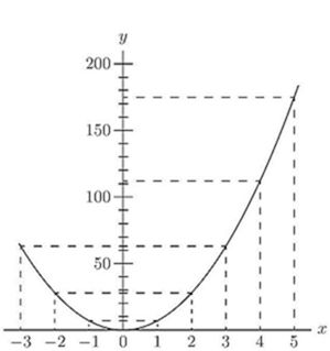
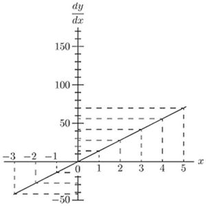
Let us illustrate this example by working out the graphs of the equations and , by assigning to a set of successive values, 0, 1, 2, 3, etc., and finding the corresponding values of and of .
These values we tabulate as follows:
| 0 | 1 | 2 | 3 | 4 | 5 | -1 | -2 | -3 | |
| 0 | 7 | 28 | 63 | 112 | 175 | 7 | 28 | 63 | |
| 0 | 14 | 28 | 42 | 56 | 70 | -14 | -28 | -42 |
Now plot these values to some convenient scale, and we obtain the two curves, Figs. 6 and 6a.
Carefully compare the two figures, and verify by inspection that the height of the ordinate of the derived curve, Fig. 6a, is proportional to the slope of the original curve, Fig. 6, at the corresponding value of . To the left of the origin, where the original curve slopes negatively (that is, downward from left to right) the corresponding ordinates of the derived curve are negative.
Footnote: See p. 76 about slopes of curves.
Now if we look back at p. 18, we shall see that simply differentiating gives us . So that the differential coefficient of is just 7 times as big as that of . If we had taken , the differential coefficient would have come out eight times as great as that of . If we put , we shall get
If we had begun with , we should have had . So that any mere multiplication by a constant reappears as a mere multiplication when the thing is differentiated. And, what is true about multiplication is equally true about division: for if, in the example above, we had taken as the constant instead of 7, we should have had the same come out in the result after differentiation.
The following further examples, fully worked out, will enable you to master completely the process of differentiation as applied to ordinary algebraical expressions, and enable you to work out by yourself the examples given at the end of this chapter.
(1) Differentiate .
is an added constant and vanishes (see p. 25).
We may then write at once
(2) Differentiate .
The term vanishes, being an added constant; and as , in the index form, is written , we have
(3) If ,
find the differential coefficient of with respect to .
As a rule an expression of this kind will need a little more knowledge than we have acquired so far; it is, however, always worth while to try whether the expression can be put in a simpler form.
First we must try to bring it into the form some expression involving only.
The expression may be written
Squaring, we get which simplifies to or that is hence
(4) The volume of a cylinder of radius and height is given by the formula . Find the rate of variation of volume with the radius when . and . If , find the dimensions of the cylinder so that a change of 1 in. in radius causes a change of 400 cub. in. in the volume.
The rate of variation of with regard to is
If and this becomes 690.8. It means that a change of radius of 1 inch will cause a change of volume of 690.8 cub. inch. This can be easily verified, for the volumes with and are 1570 cub. in. and 2260.8 cub. in. respectively, and .
Also, if
(5) The reading of a Féry's Radiation pyrometer is related to the Centigrade temperature of the observed body by the relation where is the reading corresponding to a known temperature of the observed body.
Compare the sensitiveness of the pyrometer at temperatures , given that it read 25 when the temperature was .
The sensitiveness is the rate of variation of the reading with the temperature, that is . The formula may be written and we have
When and 1200, we get and 0.1728 respectively.
The sensitiveness is approximately doubled from to , and becomes three-quarters as great again up to .
Exercises II. (See p. 252 for Answers.)
Differentiate the following:
(1) .
(2) .
(3) .
(4) .
(5) .
(6) .
Make up some other examples for yourself, and try your hand at differentiating them.
(7) If and be the lengths of a rod of iron at the temperatures . and . respectively, then . Find the change of length of the rod per degree Centigrade.
(8) It has been found that if be the candle power of an incandescent electric lamp, and be the voltage, , where and are constants.
Find the rate of change of the candle power with the voltage, and calculate the change of candle power per volt at 80,100 and 120 volts in the case of a lamp for which and .
(9) The frequency of vibration of a string of diameter , length and specific gravity , stretched with a force , is given by
Find the rate of change of the frequency when and are varied singly.
(10) The greatest external pressure which a tube can support without collapsing is given by where and are constants, is the thickness of the tube and is its diameter. (This formula assumes that is small compared to .)
Compare the rate at which varies for a small change of thickness and for a small change of diameter taking place separately.
(11) Find, from first principles, the rate at which the following vary with respect to a change in radius:
(a) the circumference of a circle of radius ;
(b) the area of a circle of radius ;
(c) the lateral area of a cone of slant dimension ;
(d) the volume of a cone of radius and height ;
(e) the area of a sphere of radius ;
(f) the volume of a sphere of radius .
(12) The length of an iron rod at the temperature being given by , where is the length at the temperature , find the rate of variation of the diameter of an iron tyre suitable for being shrunk on a wheel, when the temperature varies.
WE have learned how to differentiate simple algebraical functions such as or , and we have now to consider how to tackle the sum of two or more functions.
For instance, let what will its be? How are we to go to work on this new job?
The answer to this question is quite simple: just differentiate them, one after the other, thus:
If you have any doubt whether this is right, try a more general case, working it by first principles. And this is the way.
Let , where is any function of , and any other function of . Then, letting increase to will increase to ; and will increase to ; and to .
And we shall have:
Subtracting the original , we get and dividing through by , we get:
This justifies the procedure. You differentiate each function separately and add the results. So if now we take the example of the preceding paragraph, and put in the values of the two functions, we shall have, using the notation shown (p. 16), exactly as before.
If there were three functions of , which we may call and , so that
As for subtraction, it follows at once; for if the function had itself had a negative sign, its differential coefficient would also be negative; so that by differentiating
But when we come to do with Products, the thing is not quite so simple.
Suppose we were asked to differentiate the expression what are we to do? The result will certainly not be ; for it is easy to see that neither , nor , would have been taken into that product.
Now there are two ways in which we may go to work.
First way. Do the multiplying first, and, having worked it out, then differentiate.
Accordingly, we multiply together and .
This gives .
Now differentiate, and we get:
Second way. Go back to first principles, and consider the equation where is one function of , and is any other function of . Then, if grows to be ; and to ; and becomes , and becomes , we shall have:
Now is a small quantity of the second order of smallness, and therefore in the limit may be discarded, leaving
Then, subtracting the original , we have left and, dividing through by , we get the result:
This shows that our instructions will be as follows: To differentiate the product of two functions, multiply each function by the differential coefficient of the other, and add together the two products so obtained.
You should note that this process amounts to the following: Treat as constant while you differentiate ; then treat as constant while you differentiate ; and the whole differential coefficient will be the sum of these two treatments.
Now, having found this rule, apply it to the concrete example which was considered above.
We want to differentiate the product
Call and .
Then, by the general rule just established, we may write: exactly as before.
Lastly, we have to differentiate quotients.
Think of this example, . In such a case it is no use to try to work out the division beforehand, because will not divide into , neither have they any common factor. So there is nothing for it but to go back to first principles, and find a rule.
So we will put ;
where and are two different functions of the independent variable . Then, when becomes will become ; and will become ; and will become . So then
Now perform the algebraic division, thus:
As both these remainders are small quantities of the second order, they may be neglected, and the division may stop here, since any further remainders would be of still smaller magnitudes.
So we have got: which may be written
Now subtract the original , and we have left:
This gives us our instructions as to how to differentiate a quotient of two functions. Multiply the divisor function by the differential coefficient of the dividend function; then multiply the dividend function by the differential coefficient of the divisor function; and subtract. Lastly divide by the square of the divisor function.
Going back to our example , and
Then
The working out of quotients is often tedious, but there is nothing difficult about it.
Some further examples fully worked out are given hereafter.
(1) Differentiate .
Being a constant, vanishes, and we have
But ; so we get:
(2) Differentiate .
Putting in the index form, we get
Now
(3) Differentiate .
This may be written: .
The vanishes, and we have or, or,
(4) Differentiate .
A direct way of doing this will be explained later (see p. 66); but we can nevertheless manage it now without any difficulty.
Developing the cube, we get hence
(5) Differentiate . or, more simply, multiply out and then differentiate.
(6) Differentiate .
Same remarks as for preceding example.
(7) Differentiate .
This may be written
This, again, could be obtained more simply by multiplying the two factors first, and differentiating afterwards. This is not, however, always possible; see, for instance, p. 170, example 8, in which the rule for differentiating a product must be used.
(8) Differentiate .
(9) Differentiate .
(10) Differentiate .
In the indexed form, . hence
(11) Differentiate
Now
(12) A reservoir of square cross-section has sides sloping at an angle of with the vertical. The side of the bottom is 200 feet. Find an expression for the quantity pouring in or out when the depth of water varies by 1 foot; hence find, in gallons, the quantity withdrawn hourly when the depth is reduced from 14 to 10 feet in 24 hours.
The volume of a frustum of pyramid of height , and of bases and , is . It is easily seen that, the slope being , if the depth be , the length of the side of the square surface of the water is feet, so that the volume of water is
cubic feet per foot of depth variation. The mean level from 14 to 10 feet is 12 feet, when , , 176 cubic feet.
Gallons per hour corresponding to a change of depth of 4 ft. in 24 hours gallons.
(13) The absolute pressure, in atmospheres, , of saturated steam at the temperature . is given by Dulong as being as long as is above . Find the rate of variation of the pressure with the temperature at .
Expand the numerator by the binomial theorem (see p. 137).
hence when this becomes 0.036 atmosphere per degree Centigrade change of temperature.
Exercises III. (See the Answers on p. 253.)
(a) .
(b) .
(c) .
(d) .
(2) If , find .
(3) Find the differential coefficient of
(4) Differentiate
(5) If , find .
(6) Differentiate .
Find the differential coefficients of
(7) .
(8) .
(9) .
(10) .
(11) The temperature of the filament of an incandescent electric lamp is connected to the current passing through the lamp by the relation
Find an expression giving the variation of the current corresponding to a variation of temperature.
(12) The following formulae have been proposed to express the relation between the electric resistance of a wire at the temperature , and the resistance of that same wire at Centigrade, being constants.
Find the rate of variation of the resistance with regard to temperature as given by each of these formulae.
(13) The electromotive-force of a certain type of standard cell has been found to vary with the temperature according to the relation
Find the change of electromotive-force per degree, at , and .
(14) The electromotive-force necessary to maintain an electric arc of length with a current of intensity has been found by Mrs. Ayrton to be where are constants.
Find an expression for the variation of the electromotive-force (a) with regard to the length of the arc; (b) with regard to the strength of the current.
LET us try the effect of repeating several times over the operation of differentiating a function (see p. 13). Begin with a concrete case.
Let .
There is a certain notation, with which we are already acquainted (see p. 14), used by some writers, that is very convenient. This is to employ the general symbol for any function of . Here the symbol is read as "function of," without saying what particular function is meant. So the statement merely tells us that is a function of , it may be or , or or any other complicated function of .
The corresponding symbol for the differential coefficient is , which is simpler to write than . This is called the "derived function" of .
Suppose we differentiate over again, we shall get the "second derived function" or second differential coefficient, which is denoted by ; and so on.
Now let us generalize.
Let .
But this is not the only way of indicating successive differentiations.
For, and this is more conveniently written as , or more usually .
Similarly, we may write as the result of thrice differentiating, .
Now let us try .
In a similar manner if ,
Exercises IV. (See page 253 for Answers.)
Find and for the following expressions:
(1) .
(2) .
(3) .
(4) Find the 2nd and 3rd derived functions in the Exercises III. (p. 45), No. 1 to No. 7, and in the Examples given (p. 40), No. 1 to No. 7.
SOME of the most important problems of the calculus are those where time is the independent variable, and we have to think about the values of some other quantity that varies when the time varies. Some things grow larger as time goes on; some other things grow smaller. The distance that a train has got from its starting place goes on ever increasing as time goes on. Trees grow taller as the years go by. Which is growing at the greater rate; a plant 12 inches high which in one month becomes 14 inches high, or a tree 12 feet high which in a year becomes 14 feet high?
In this chapter we are going to make much use of the word rate. Nothing to do with poor-rate, or water-rate (except that even here the word suggests a proportion—a ratio—so many pence in the pound). Nothing to do even with birth-rate or death-rate, though these words suggest so many births or deaths per thousand of the population. When a motor-car whizzes by us, we say: What a terrific rate! When a spendthrift is flinging about his money, we remark that that young man is living at a prodigious rate. What do we mean by rate? In both these cases we are making a mental comparison of something that is happening, and the length of time that it takes to happen. If the motor-car flies past us going 10 yards per second, a simple bit of mental arithmetic will show us that this is equivalent—while it lasts—to a rate of 600 yards per minute, or over 20 miles per hour.
Now in what sense is it true that a speed of 10 yards per second is the same as 600 yards per minute? Ten yards is not the same as 600 yards, nor is one second the same thing as one minute. What we mean by saying that the rate is the same, is this: that the proportion borne between distance passed over and time taken to pass over it, is the same in both cases.
Take another example. A man may have only a few pounds in his possession, and yet be able to spend money at the rate of millions a year-provided he goes on spending money at that rate for a few minutes only. Suppose you hand a shilling over the counter to pay for some goods; and suppose the operation lasts exactly one second. Then, during that brief operation, you are parting with your money at the rate of 1 shilling per second, which is the same rate as per minute, or per hour, or per day, or per year! If you have in your pocket, you can go on spending money at the rate of a million a year for just minutes.
It is said that Sandy had not been in London above five minutes when "bang went saxpence." If he were to spend money at that rate all day long, say for 12 hours, he would be spending 6 shillings an hour, or per day, or a week, not counting the Sawbbath.
Now try to put some of these ideas into differential notation.
Let in this case stand for money, and let stand for time.
If you are spending money, and the amount you spend in a short time be called , the rate of spending it will be , or rather, should be written with a minus sign, as , because is a decrement, not an increment. But money is not a good example for the calculus, because it generally comes and goes by jumps, not by a continuous flow-you may earn a year, but it does not keep running in all day long in a thin stream; it comes in only weekly, or monthly, or quarterly, in lumps: and your expenditure also goes out in sudden payments.
A more apt illustration of the idea of a rate is furnished by the speed of a moving body. From London (Euston station) to Liverpool is 200 miles. If a train leaves London at 7 o'clock, and reaches Liverpool at 11 o'clock, you know that, since it has travelled 200 miles in 4 hours, its average rate must have been 50 miles per hour; because . Here you are really making a mental comparison between the distance passed over and the time taken to pass over it. You are dividing one by the other. If is the whole distance, and the whole time, clearly the average rate is . Now the speed was not actually constant all the way: at starting, and during the slowing up at the end of the journey, the speed was less. Probably at some part, when running downhill, the speed was over 60 miles an hour. If, during any particular element of time , the corresponding element of distance passed over was , then at that part of the journey the speed was . The rate at which one quantity (in the present instance, distance) is changing in relation to the other quantity (in this case, time) is properly expressed, then, by stating the differential coefficient of one with respect to the other. A velocity, scientifically expressed, is the rate at which a very small distance in any given direction is being passed over; and may therefore be written
But if the velocity is not uniform, then it must be either increasing or else decreasing. The rate at which a velocity is increasing is called the acceleration. If a moving body is, at any particular instant, gaining an additional velocity in an element of time , then the acceleration at that instant may be written but is itself . Hence we may put and this is usually written ; or the acceleration is the second differential coefficient of the distance, with respect to time. Acceleration is expressed as a change of velocity in unit time, for instance, as being so many feet per second per second; the notation used being feet .
When a railway train has just begun to move, its velocity is small; but it is rapidly gaining speed-it is being hurried up, or accelerated, by the effort of the engine. So its is large. When it has got up its top speed it is no longer being accelerated, so that then has fallen to zero. But when it nears its stopping place its speed begins to slow down; may, indeed, slow down very quickly if the brakes are put on, and during this period of deceleration or slackening of pace, the value of , that is, of will be negative.
To accelerate a mass requires the continuous application of force. The force necessary to accelerate a mass is proportional to the mass, and it is also proportional to the acceleration which is being imparted. Hence we may write for the force , the expression
The product of a mass by the speed at which it is going is called its momentum, and is in symbols . If we differentiate momentum with respect to time we shall get for the rate of change of momentum. But, since is a constant quantity, this may be written , which we see above is the same as . That is to say, force may be expressed either as mass times acceleration, or as rate of change of momentum.
Again, if a force is employed to move something (against an equal and opposite counter-force), it does work; and the amount of work done is measured by the product of the force into the distance (in its own direction) through which its point of application moves forward. So if a force moves forward through a length , the work done (which we may call ) will be where we take as a constant force. If the force varies at different parts of the range , then we must find an expression for its value from point to point. If be the force along the small element of length , the amount of work done will be . But as is only an element of length, only an element of work will be done. If we write for work, then an element of work will be ; and we have which may be written
Further, we may transpose the expression and write
This gives us yet a third definition of force; that if it is being used to produce a displacement in any direction, the force (in that direction) is equal to the rate at which work is being done per unit of length in that direction. In this last sentence the word rate is clearly not used in its time-sense, but in its meaning as ratio or proportion.
Sir Isaac Newton, who was (along with Leibnitz) an inventor of the methods of the calculus, regarded all quantities that were varying as flowing; and the ratio which we nowadays call the differential coefficient he regarded as the rate of flowing, or the fluxion of the quantity in question. He did not use the notation of the and , and (this was due to Leibnitz), but had instead a notation of his own. If was a quantity that varied, or "flowed," then his symbol for its rate of variation (or "fluxion") was . If was the variable, then its fluxion was called . The dot over the letter indicated that it had been differentiated. But this notation does not tell us what is the independent variable with respect to which the differentiation has been effected. When we see we know that is to be differentiated with respect to . If we see we know that is to be differentiated with respect to . But if we see merely , we cannot tell without looking at the context whether this is to mean or or , or what is the other variable. So, therefore, this fluxional notation is less informing than the differential notation, and has in consequence largely dropped out of use. But its simplicity gives it an advantage if only we will agree to use it for those cases exclusively where time is the independent variable. In that case will mean and will mean ; and will mean .
Adopting this fluxional notation we may write the mechanical equations considered in the paragraphs above, as follows:
(1) A body moves so that the distance (in feet), which it travels from a certain point , is given by the relation , where is the time in seconds elapsed since a certain instant. Find the velocity and acceleration 5 seconds after the body began to move, and also find the corresponding values when the distance covered is 100 feet. Find also the average velocity during the first 10 seconds of its motion. (Suppose distances and motion to the right to be positive.)
Now
When and . The body started from a point 10.4 feet to the right of the point ; and the time was reckoned from the instant the body started.
When .
When , or , and ; .
When ,
(It is the same velocity as the velocity at the middle of the interval, ; for, the acceleration being constant, the velocity has varied uniformly from zero when to when .)
(2) In the above problem let us suppose
When and , the time is reckoned from the instant at which the body passed a point 10.4 ft. from the point , its velocity being then already . To find the time elapsed since it began moving, let ; then . The body began moving 7.5 sec. before time was begun to be observed; 5 seconds after this gives and .
When , hence .
To find the distance travelled during the 10 first seconds of the motion one must know how far the body was from the point when it started.
When , that is 0.85 ft. to the left of the point .
Now, when ,
So, in 10 seconds, the distance travelled was , and
(3) Consider a similar problem when the distance is given by . Then constant. When , as before, and ; so that the body was moving in the direction opposite to its motion in the previous cases. As the acceleration is positive, however, we see that this velocity will decrease as time goes on, until it becomes zero, when or ; or . After this, the velocity becomes positive; and 5 seconds after the body started, , and
When ,
When is zero, , informing us that the body moves back to 0.85 ft. beyond the point before it stops. Ten seconds later
The distance travelled , and the average velocity is again 2 ft./sec.
(4) Consider yet another problem of the same sort with . The acceleration is no more constant.
When . The body is at rest, but just ready to move with a negative acceleration, that is to gain a velocity towards the point .
(5) If we have , then , and .
When .
The body is moving towards the point with a velocity of , and just at that instant the velocity is uniform.
We see that the conditions of the motion can always be at once ascertained from the time-distance equation and its first and second derived functions. In the last two cases the mean velocity during the first 10 seconds and the velocity 5 seconds after the start will no more be the same, because the velocity is not increasing uniformly, the acceleration being no longer constant.
(6) The angle (in radians) turned through by a wheel is given by , where is the time in seconds from a certain instant; find the angular velocity and the angular acceleration , (a) after 1 second; (b) after it has performed one revolution. At what time is it at rest, and how many revolutions has it performed up to that instant?
Writing for the acceleration
When .
When ,
This is a retardation; the wheel is slowing down.
After 1 revolution
By plotting the graph, , we can get the value or values of for which ; these are 2.11 and 3.03 (there is a third negative value).
When ,
When ,
The velocity is reversed. The wheel is evidently at rest between these two instants; it is at rest when , that is when , or when , it has performed
Exercises V. (See page 255 for Answers.)
(1) If ; find and .
(2) A body falling freely in space describes in seconds a space , in feet, expressed by the equation . Draw a curve showing the relation between and . Also determine the velocity of the body at the following times from its being let drop: seconds; seconds; second.
(3) If ; find and .
(4) If a body move according to the law find its velocity when seconds; being in feet.
(5) Find the acceleration of the body mentioned in the preceding example. Is the acceleration the same for all values of ?
(6) The angle (in radians) turned through by a revolving wheel is connected with the time (in seconds) that has elapsed since starting; by the law
Find the angular velocity (in radians per second) of that wheel when seconds have elapsed. Find also its angular acceleration.
(7) A slider moves so that, during the first part of its motion, its distance in inches from its starting point is given by the expression
Find the expression for the velocity and the acceleration at any time; and hence find the velocity and the acceleration after 3 seconds.
(8) The motion of a rising balloon is such that its height , in miles, is given at any instant by the expression ; being in seconds.
Find an expression for the velocity and the acceleration at any time. Draw curves to show the variation of height, velocity and acceleration during the first ten minutes of the ascent.
(9) A stone is thrown downwards into water and its depth in metres at any instant seconds after reaching the surface of the water is given by the expression
Find an expression for the velocity and the acceleration at any time. Find the velocity and acceleration after 10 seconds.
(10) A body moves in such a way that the spaces described in the time from starting is given by , where is a constant. Find the value of when the velocity is doubled from the 5th to the 10th second; find it also when the velocity is numerically equal to the acceleration at the end of the 10th second.
SOMETIMES one is stumped by finding that the expression to be differentiated is too complicated to tackle directly.
Thus, the equation is awkward to a beginner.
Now the dodge to turn the difficulty is this: Write some symbol, such as , for the expression ; then the equation becomes which you can easily manage; for
Then tackle the expression and differentiate it with respect to ,
Then all that remains is plain sailing; that is, and so the trick is done.
By and bye, when you have learned how to deal with sines, and cosines, and exponentials, you will find this dodge of increasing usefulness.
Let us practise this dodge on a few examples.
(1) Differentiate .
Let .
(2) Differentiate .
Let .
(3) Differentiate .
Let .
(4) Differentiate .
Let .
(5) Differentiate .
Write this as . (We may also write and differentiate as a product.)
Proceeding as in example (1) above, we get
Hence or
(6) Differentiate .
We may write this
Differentiating , as shown in example (2) above, we get so that
(7) Differentiate .
Let .
Now let and .
Hence ,
(8) Differentiate .
We get
Let and .
Let and .
Hence
(9) Differentiate with respect to . (10) Find the first and second differential coefficients of .
Let and let ; then .
Hence
Now (We shall need these two last differential coefficients later on. See Ex. X. No. 11.)
Exercises VI. (See page 255 for Answers.)
Differentiate the following:
(1) .
(2) .
(3) .
(4) .
(5) .
(6) .
(7) .
(8) Differentiate with respect to .
(9) Differentiate .
The process can be extended to three or more differential coefficients, so that .
(1) If , find .
We have
(2) If , find .
Hence an expression in which must be replaced by its value, and by its value in terms of .
(3) If and , find .
We get (see example 5, p. 68); and
So that .
Replace now first , then by its value.
Exercises VII. You can now successfully try the following. (See page 256 for Answers.)
(1) If and , find .
(2) If and , find .
(3) If and , find .
IT is useful to consider what geometrical meaning can be given to the differential coefficient.
In the first place, any function of , such, for example, as , or , or , can be plotted as a curve; and nowadays every schoolboy is familiar with the process of curve-plotting.
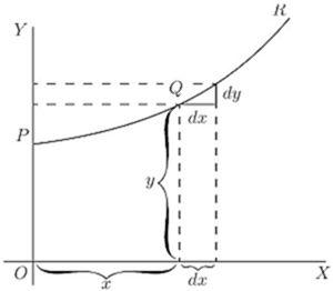
Let , in Fig. 7, be a portion of a curve plotted with respect to the axes of coordinates and . Consider any point on this curve, where the abscissa of the point is and its ordinate is . Now observe how changes when is varied. If is made to increase by a small increment , to the right, it will be observed that also (in this particular curve) increases by a small increment (because this particular curve happens to be an ascending curve). Then the ratio of to is a measure of the degree to which the curve is sloping up between the two points and . As a matter of fact, it can be seen on the figure that the curve between and has many different slopes, so that we cannot very well speak of the slope of the curve between and . If, however, and are so near each other that the small portion of the curve is practically straight, then it is true to say that the ratio is the slope of the curve along . The straight line produced on either side touches the curve along the portion only, and if this portion is indefinitely small, the straight line will touch the curve at practically one point only, and be therefore a tangent to the curve.
This tangent to the curve has evidently the same slope as , so that is the slope of the tangent to the curve at the point for which the value of is found.
We have seen that the short expression "the slope of a curve" has no precise meaning, because a curve has so many slopes-in fact, every small portion of a curve has a different slope. "The slope of a curve at a point" is, however, a perfectly defined thing; it is the slope of a very small portion of the curve situated just at that point; and we have seen that this is the same as "the slope of the tangent to the curve at that point."
Observe that is a short step to the right, and the corresponding short step upwards. These steps must be considered as short as possible—in fact indefinitely short,—though in diagrams we have to represent them by bits that are not infinitesimally small, otherwise they could not be seen.
We shall hereafter make considerable use of this circumstance that represents the slope of the curve at any point.
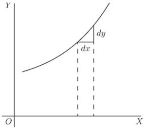
If a curve is sloping up at at a particular point, as in Fig. 8, and will be equal, and the value of .
If the curve slopes up steeper than (Fig. 9), will be greater than 1.
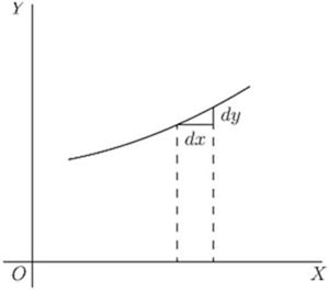
If the curve slopes up very gently, as in Fig. 10, will be a fraction smaller than 1.
For a horizontal line, or a horizontal place in a curve, , and therefore .
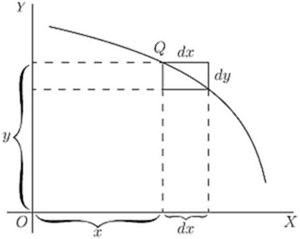
If a curve slopes downward, as in Fig. 11, will be a step down, and must therefore be reckoned of negative value; hence will have negative sign also.
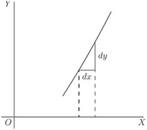
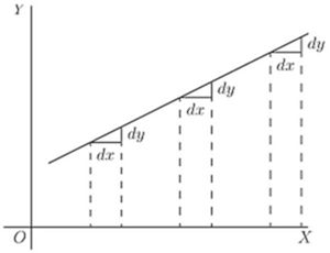
If the "curve" happens to be a straight line, like that in Fig. 12, the value of will be the same at all points along it. In other words its slope is constant.
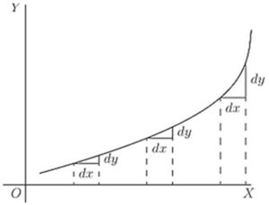
If a curve is one that turns more upwards as it goes along to the right, the values of will become greater and greater with the increasing steepness, as in Fig. 13.
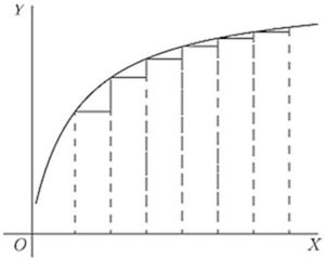
If a curve is one that gets flatter and flatter as it goes along, the values of will become smaller and smaller as the flatter part is reached, as in Fig. 14.
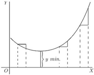
If a curve first descends, and then goes up again, as in Fig. 15, presenting a concavity upwards, then clearly will first be negative, with diminishing values as the curve flattens, then will be zero at the point where the bottom of the trough of the curve is reached; and from this point onward will have positive values that go on increasing. In such a case is said to pass by a minimum.
The minimum value of is not necessarily the smallest value of , it is that value of corresponding to the bottom of the trough; for instance, in Fig. 28 (p. 99), the value of corresponding to the bottom of the trough is 1, while takes elsewhere values which are smaller than this. The characteristic of a minimum is that must increase on either side of it.
N.B.—For the particular value of that makes a minimum, the value of .
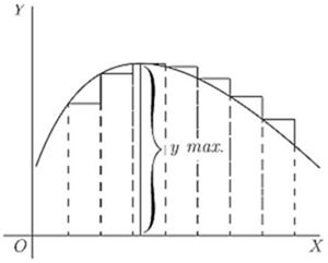
If a curve first ascends and then descends, the values of will be positive at first; then zero, as the summit is reached; then negative, as the curve slopes downwards, as in Fig. 16. In this case is said to pass by a maximum, but the maximum value of is not necessarily the greatest value of . In Fig. 28, the maximum of is , but this is by no means the greatest value can have at some other point of the curve.
N.B.—For the particular value of that makes a maximum, the value of .
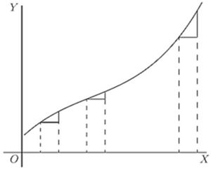
If a curve has the peculiar form of Fig. 17, the values of will always be positive; but there will be one particular place where the slope is least steep, where the value of will be a minimum; that is, less than it is at any other part of the curve.
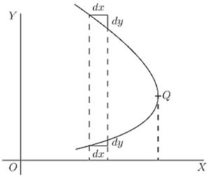
If a curve has the form of Fig. 18, the value of will be negative in the upper part, and positive in the lower part; while at the nose of the curve where it becomes actually perpendicular, the value of will be infinitely great.
Now that we understand that measures the steepness of a curve at any point, let us turn to some of the equations which we have already learned how to differentiate.
(1) As the simplest case take this:
It is plotted out in Fig. 19, using equal scales for and . If we put , then the corresponding ordinate will be ; that is to say, the "curve" crosses the -axis at the height . From here it ascends at ; for whatever values we give to to the right, we have an equal to ascend. The line has a gradient of 1 in 1.
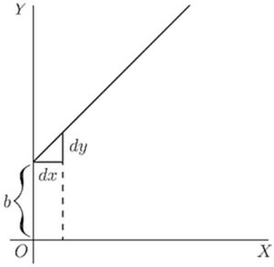
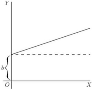
Now differentiate , by the rules we have already learned (pp. 21 and 25 ante), and we get .
The slope of the line is such that for every little step to the right, we go an equal little step upward. And this slope is constant-always the same slope.
(2) Take another case:
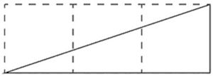
We know that this curve, like the preceding one, will start from a height on the -axis. But before we draw the curve, let us find its slope by differentiating; which gives . The slope will be constant, at an angle, the tangent of which is here called . Let us assign to some numerical value—say . Then we must give it such a slope that it ascends 1 in 3; or will be 3 times as great as ; as magnified in Fig. 21. So, draw the line in Fig. 20 at this slope.
(3) Now for a slightly harder case.
Let
Again the curve will start on the -axis at a height above the origin.
Now differentiate. [If you have forgotten, turn back to p. 25; or, rather, don't turn back, but think out the differentiation.]
This shows that the steepness will not be constant: it increases as increases. At the starting point , where , the curve (Fig. 22) has no steepness—that is, it is level. On the left of the origin, where has negative values, will also have negative values, or will descend from left to right, as in the Figure.
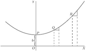
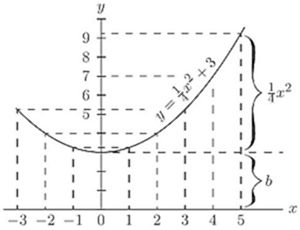
Let us illustrate this by working out a particular instance. Taking the equation and differentiating it, we get
Now assign a few successive values, say from 0 to 5, to ; and calculate the corresponding values of by the first equation; and of from the second equation. Tabulating results, we have:
| 0 | 1 | 2 | 3 | 4 | 5 | |
| 3 | 4 | 7 | ||||
| 0 | 1 | 2 |
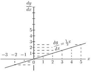
Then plot them out in two curves, Figs. 23 and 24, in Fig. 23 plotting the values of against those of and in Fig. 24 those of against those of . For any assigned value of , the height of the ordinate in the second curve is proportional to the slope of the first curve.
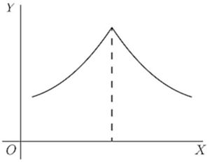
If a curve comes to a sudden cusp, as in Fig. 25, the slope at that point suddenly changes from a slope upward to a slope downward. In that case will clearly undergo an abrupt change from a positive to a negative value.
The following examples show further applications of the principles just explained.
(4) Find the slope of the tangent to the curve at the point where . Find the angle which this tangent makes with the curve .
The slope of the tangent is the slope of the curve at the point where they touch one another (see p. 76); that is, it is the of the curve for that point. Here and for , which is the slope of the tangent and of the curve at that point. The tangent, being a straight line, has for equation , and its slope is , hence . Also if ; and as the tangent passes by this point, the coordinates of the point must satisfy the equation of the tangent, namely so that and ; the equation of the tangent is therefore .
Now, when two curves meet, the intersection being a point common to both curves, its coordinates must satisfy the equation of each one of the two curves; that is, it must be a solution of the system of simultaneous equations formed by coupling together the equations of the curves. Here the curves meet one another at points given by the solution of that is,
This equation has for its solutions and . The slope of the curve at any point is
For the point where , this slope is zero; the curve is horizontal. For the point where hence the curve at that point slopes downwards to the right at such an angle with the horizontal that ; that is, at to the horizontal.
The slope of the straight line is ; that is, it slopes downwards to the right and makes with the horizontal an angle such that ; that is, an angle of . It follows that at the first point the curve cuts the straight line at an angle of , while at the second it cuts it at an angle of .
(5) A straight line is to be drawn, through a point whose coordinates are , as tangent to the curve . Find the coordinates of the point of contact.
The slope of the tangent must be the same as the of the curve; that is, .
The equation of the straight line is , and as it is satisfied for the values , then ; also, its .
The and the of the point of contact must also satisfy both the equation of the tangent and the equation of the curve.
We have then four equations in .
Equations (i) and (ii) give .
Replacing and by their value in this, we get which simplifies to , the solutions of which are: and . Replacing in (i), we get and respectively; the two points of contact are then , , and , .
Note.—In all exercises dealing with curves, students will find it extremely instructive to verify the deductions obtained by actually plotting the curves.
Exercises VIII. (See page 256 for Answers.)
(1) Plot the curve , using a scale of millimetres. Measure at points corresponding to different values of , the angle of its slope.
Find, by differentiating the equation, the expression for slope; and see, from a Table of Natural Tangents, whether this agrees with the measured angle.
(2) Find what will be the slope of the curve
at the particular point that has as abscissa .
(3) If , show that at the particular point of the curve where will have the value .
(4) Find the of the equation ; and calculate the numerical values of for the points corresponding to , , .
(5) In the curve to which the equation is , find the values of at those points where the slope .
(6) Find the slope, at any point, of the curve whose equation is ; and give the numerical value of the slope at the place where , and at that where .
(7) The equation of a tangent to the curve , being of the form , where and are constants, find the value of and if the point where the tangent touches the curve has for abscissa.
(8) At what angle do the two curves cut one another?
(9) Tangents to the curve are drawn at points for which and . Find the coordinates of the point of intersection of the tangents and their mutual inclination.
(10) A straight line touches a curve at one point. What are the coordinates of the point of contact, and what is the value of ?
ONE of the principal uses of the process of differentiating is to find out under what conditions the value of the thing differentiated becomes a maximum, or a minimum. This is often exceedingly important in engineering questions, where it is most desirable to know what conditions will make the cost of working a minimum, or will make the efficiency a maximum.
Now, to begin with a concrete case, let us take the equation
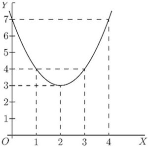
By assigning a number of successive values to , and finding the corresponding values of , we can readily see that the equation represents a curve with a minimum.
| 0 | 1 | 2 | 3 | 4 | 5 | |
| 7 | 4 | 3 | 4 | 7 | 12 |
These values are plotted in Fig. 26, which shows that has apparently a minimum value of 3, when is made equal to 2. But are you sure that the minimum occurs at 2, and not at or at ?
Of course it would be possible with any algebraic expression to work out a lot of values, and in this way arrive gradually at the particular value that may be a maximum or a minimum.
Here is another example:
Let
Calculate a few values thus:
| -1 | 0 | 1 | 2 | 3 | 4 | 5 | |
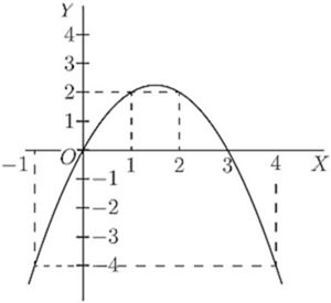
| -4 | 0 | 2 | 2 | 0 | -4 | -10 |
Plot these values as in Fig. 27.
It will be evident that there will be a maximum somewhere between and ; and the thing looks as if the maximum value of ought to be about . Try some intermediate values. If ; if ; if . How can we be sure that 2.25 is the real maximum, or that it occurs exactly when ?
Now it may sound like juggling to be assured that there is a way by which one can arrive straight at a maximum (or minimum) value without making a lot of preliminary trials or guesses. And that way depends on differentiating. Look back to an earlier page (78) for the remarks about Figs. 14 and 15, and you will see that whenever a curve gets either to its maximum or to its minimum height, at that point its . Now this gives us the clue to the dodge that is wanted. When there is put before you an equation, and you want to find that value of that will make its a minimum (or a maximum), first differentiate it, and having done so, write its as equal to zero, and then solve for . Put this particular value of into the original equation, and you will then get the required value of . This process is commonly called "equating to zero."
To see how simply it works, take the example with which this chapter opens, namely
Differentiating, we get: Now equate this to zero, thus: Solving this equation for , we get:
Now, we know that the maximum (or minimum) will occur exactly when .
Putting the value into the original equation, we get
Now look back at Fig. 26, and you will see that the minimum occurs when , and that this minimum of .
Try the second example (Fig. 24), which is
Differentiating, .
Equating to zero, and putting this value of into the original equation, we find: This gives us exactly the information as to which the method of trying a lot of values left us uncertain.
Now, before we go on to any further cases, we have two remarks to make. When you are told to equate to zero, you feel at first (that is if you have any wits of your own) a kind of resentment, because you know that has all sorts of different values at different parts of the curve, according to whether it is sloping up or down. So, when you are suddenly told to write you resent it, and feel inclined to say that it can't be true. Now you will have to understand the essential difference between "an equation," and "an equation of condition." Ordinarily you are dealing with equations that are true in themselves, but, on occasions, of which the present are examples, you have to write down equations that are not necessarily true, but are only true if certain conditions are to be fulfilled; and you write them down in order, by solving them, to find the conditions which make them true. Now we want to find the particular value that has when the curve is neither sloping up nor sloping down, that is, at the particular place where . So, writing does not mean that it always is ; but you write it down as a condition in order to see how much will come out if is to be zero.
The second remark is one which (if you have any wits of your own) you will probably have already made: namely, that this much-belauded process of equating to zero entirely fails to tell you whether the that you thereby find is going to give you a maximum value of or a minimum value of . Quite so. It does not of itself discriminate; it finds for you the right value of but leaves you to find out for yourselves whether the corresponding is a maximum or a minimum. Of course, if you have plotted the curve, you know already which it will be.
For instance, take the equation:
Without stopping to think what curve it corresponds to, differentiate it, and equate to zero: whence and, inserting this value, will be either a maximum or else a minimum. But which? You will hereafter be told a way, depending upon a second differentiation, (see Chap. XII., p. 109). But at present it is enough if you will simply try any other value of differing a little from the one found, and see whether with this altered value the corresponding value of is less or greater than that already found.
Try another simple problem in maxima and minima. Suppose you were asked to divide any number into two parts, such that the product was a maximum? How would you set about it if you did not know the trick of equating to zero? I suppose you could worry it out by the rule of try, try, try again. Let 60 be the number. You can try cutting it into two parts, and multiplying them together. Thus, 50 times 10 is 500; 52 times 8 is 416; 40 times 20 is 800; 45 times 15 is 675; 30 times 30 is 900. This looks like a maximum: try varying it. 31 times 29 is 899, which is not so good; and 32 times 28 is 896, which is worse. So it seems that the biggest product will be got by dividing into two equal halves.
Now see what the calculus tells you. Let the number to be cut into two parts be called . Then if is one part, the other will be , and the product will be or . So we write . Now differentiate and equate to zero; Solving for , we get .
So now we know that whatever number may be, we must divide it into two equal parts if the product of the parts is to be a maximum; and the value of that maximum product will always be .
This is a very useful rule, and applies to any number of factors, so that if a constant number, is a maximum when .
Let us at once apply our knowledge to a case that we can test.
Let and let us find whether this function has a maximum or minimum; and if so, test whether it is a maximum or a minimum.
Differentiating, we get
Equating to zero, we get whence or
That is to say, when is made , the corresponding value of will be either a maximum or a minimum. Accordingly, putting in the original equation, we get
Is this a maximum or a minimum? To test it, try putting a little bigger than ,—say make . Then which is higher up than -0.25; showing that is a minimum.
Plot the curve for yourself, and verify the calculation.
A most interesting example is afforded by a curve that has both a maximum and a minimum. Its equation is: Now
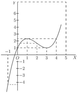
Equating to zero, we get the quadratic, and solving the quadratic gives us two roots, viz.
Now, when ; and when . The first of these is a minimum, the second a maximum.
The curve itself may be plotted (as in Fig. 28) from the values calculated, as below, from the original equation.
| -1 | 0 | 1 | 2 | 3 | 4 | 5 | 6 | |
| 1 | 1 | 19 |
A further exercise in maxima and minima is afforded by the following example:
The equation to a circle of radius , having its centre at the point whose coordinates are , as depicted in Fig. 29, is:
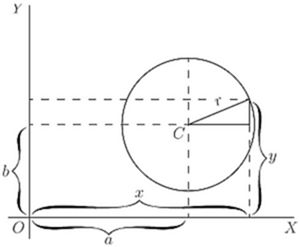
This may be transformed into
Now we know beforehand, by mere inspection of the figure, that when , will be either at its maximum value, , or else at its minimum value, . But let us not take advantage of this knowledge; let us set about finding what value of will make a maximum or a minimum, by the process of differentiating and equating to zero. which reduces to
Then the condition for being maximum or minimum is:
Since no value whatever of will make the denominator infinite, the only condition to give zero is
Inserting this value in the original equation for the circle, we find and as the root of is either or , we have two resulting values of ,
The first of these is the maximum, at the top; the second the minimum, at the bottom.
If the curve is such that there is no place that is a maximum or minimum, the process of equating to zero will yield an impossible result. For instance:
Let
Then
Equating this to zero, we get , Therefore has no maximum nor minimum.
A few more worked examples will enable you to thoroughly master this most interesting and useful application of the calculus.
(1) What are the sides of the rectangle of maximum area inscribed in a circle of radius ?
If one side be called , and as the diagonal of the rectangle is necessarily a diameter, the other side .
Then, area of rectangle ,
If you have forgotten how to differentiate , here is a hint: write and , and seek and ; fight it out, and only if you can't get on refer to page 66.
You will get
For maximum or minimum we must have that is, and .
The other side ; the two sides are equal; the figure is a square the side of which is equal to the diagonal of the square constructed on the radius. In this case it is, of course, a maximum with which we are dealing.
(2) What is the radius of the opening of a conical vessel the sloping side of which has a length when the capacity of the vessel is greatest?
If be the radius and the corresponding height, .
Proceeding as in the previous problem, we get for maximum or minimum.
Or, , and , for a maximum, obviously.
(3) Find the maxima and minima of the function
We get for maximum or minimum; or
There is only one value, hence only one maximum or minimum. it is therefore a minimum. (It is instructive to plot the graph of the function.)
(4) Find the maxima and minima of the function . (It will be found instructive to plot the graph.)
Differentiating gives at once (see example No. 1, p. 67) for maximum or minimum.
Hence and , the only solution. For .
For , so this is a maximum.
(5) Find the maxima and minima of the function
We have for maximum or minimum; or or ; which has for solutions
These being imaginary, there is no real value of for which ; hence there is neither maximum nor minimum.
(6) Find the maxima and minima of the function
This may be written . that is, , which is satisfied for , and for , that is for . So there are two solutions.
Taking first . If , and if . On one side is imaginary; that is, there is no value of that can be represented by a graph; the latter is therefore entirely on the right side of the axis of (see Fig. 30).
On plotting the graph it will be found that the curve goes to the origin, as if there were a minimum there; but instead of continuing beyond, as it should do for a minimum, it retraces its steps (forming what is called a "cusp"). There is no minimum, therefore, although the condition for a minimum is satisfied, namely . It is necessary therefore always to check by taking one value on either side.
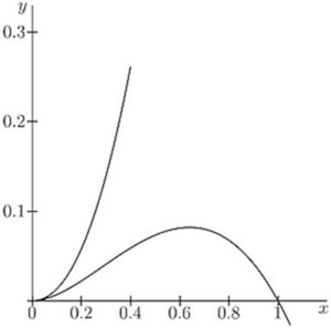
Now, if we take . If and ; if , becomes 0.6389 and 0.0811; and if , becomes 0.8996 and 0.0804.
This shows that there are two branches of the curve; the upper one does not pass through a maximum, but the lower one does.
(7) A cylinder whose height is twice the radius of the base is increasing in volume, so that all its parts keep always in the same proportion to each other; that is, at any instant, the cylinder is similar to the original cylinder. When the radius of the base is feet, the surface area is increasing at the rate of 20 square inches per second; at what rate is its volume then increasing?
The volume changes at the rate of cubic inches.
Make other examples for yourself. There are few subjects which offer such a wealth for interesting examples.
Exercises IX. (See page 257 for Answers.)
(1) What values of will make a maximum and a minimum, if ?
(2) What value of will make a maximum in the equation ?
(3) A line of length is to be cut up into 4 parts and put together as a rectangle. Show that the area of the rectangle will be a maximum if each of its sides is equal to .
(4) A piece of string 30 inches long has its two ends joined together and is stretched by 3 pegs so as to form a triangle. What is the largest triangular area that can be enclosed by the string?
(5) Plot the curve corresponding to the equation also find , and deduce the value of that will make a minimum; and find that minimum value of .
(6) If , find what values of will make a maximum or a minimum.
(7) What is the smallest square that can be inscribed in a given square?
(8) Inscribe in a given cone, the height of which is equal to the radius of the base, a cylinder (a whose volume is a maximum; (b) whose lateral area is a maximum; (c) whose total area is a maximum.
(9) Inscribe in a sphere, a cylinder (a) whose volume is a maximum; (b) whose lateral area is a maximum; (c) whose total area is a maximum.
(10) A spherical balloon is increasing in volume. If, when its radius is feet, its volume is increasing at the rate of 4 cubic feet per second, at what rate is its surface then increasing?
(11) Inscribe in a given sphere a cone whose volume is a maximum.
(12) The current given by a battery of similar voltaic cells is , where , are constants and is the number of cells coupled in series. Find the proportion of to for which the current is greatest.
RETURNING to the process of successive differentiation, it may be asked: Why does anybody want to differentiate twice over? We know that when the variable quantities are space and time, by differentiating twice over we get the acceleration of a moving body, and that in the geometrical interpretation, as applied to curves, means the slope of the curve. But what can mean in this case? Clearly it means the rate (per unit of length ) at which the slope is changing-in brief, it is a measure of the curvature of the slope.
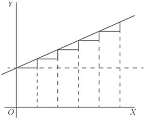
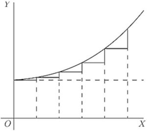
Suppose a slope constant, as in Fig. 31.
Here, is of constant value.
Suppose, however, a case in which, like Fig. 32, the slope itself is getting greater upwards, then , that is, , will be positive.
If the slope is becoming less as you go to the right (as in Fig. 14, p. 80), or as in Fig. 33, then, even though the curve may be going upward, since the change is such as to diminish its slope, its will be negative.
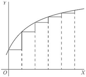
It is now time to initiate you into another secret-how to tell whether the result that you get by "equating to zero" is a maximum or a minimum. The trick is this: After you have differentiated (so as to get the expression which you equate to zero), you then differentiate a second time, and look whether the result of the second differentiation is positive or negative. If comes out positive, then you know that the value of which you got was a minimum; but if comes out negative, then the value of which you got must be a maximum. That's the rule.
The reason of it ought to be quite evident. Think of any curve that has a minimum point in it (like Fig. 15, p. 80), or like Fig. 34, where the point of minimum is marked , and the curve is concave upwards. To the left of the slope is downward, that is, negative, and is getting less negative. To the right of the slope has become upward, and is getting more and more upward. Clearly the change of slope as the curve passes through is such that is positive, for its operation, as increases toward the right, is to convert a downward slope into an upward one.
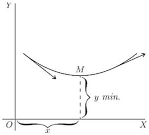
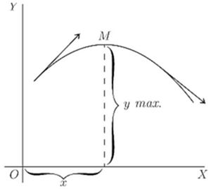
Similarly, consider any curve that has a maximum point in it (like Fig. 16, p. 81), or like Fig. 35, where the curve is convex, and the maximum point is marked . In this case, as the curve passes through from left to right, its upward slope is converted into a downward or negative slope, so that in this case the "slope of the slope" is negative.
Go back now to the examples of the last chapter and verify in this way the conclusions arrived at as to whether in any particular case there is a maximum or a minimum. You will find below a few worked out examples.
(1) Find the maximum or minimum of
(a) ;
(b) ;
and ascertain if it be a maximum or a minimum in each case.
(a) , and
; it is +; hence it is a minimum.
(b) and . it is hence it is a maximum.
(2) Find the maxima and minima of the function . hence corresponds to a minimum . For it is -; hence corresponds to a maximum .
(3) Find the maxima and minima of . or , whose solutions are and .
The denominator is always positive, so it is sufficient to ascertain the sign of the numerator.
If we put , the numerator is negative; the maximum, .
If we put , the numerator is positive; the minimum, .
(4) The expense of handling the products of a certain factory varies with the weekly output according to the relation , where are positive constants. For what output will the expense be least? hence and .
As the output cannot be negative, .
Now which is positive for all the values of ; hence corresponds to a minimum.
(5) The total cost per hour of lighting a building with lamps of a certain kind is where is the commercial efficiency (watts per candle),
Moreover, the relation connecting the average life of a lamp with the commercial efficiency at which it is run is approximately , where and are constants depending on the kind of lamp.
Find the commercial efficiency for which the total cost of lighting will be least.
We have for maximum or minimum.
This is clearly for minimum, since which is positive for a positive value of .
For a particular type of 16 candle-power lamps, pence, pence; and it was found that and .
Exercises X. (You are advised to plot the graph of any numerical example.) (See p. 258 for the Answers.)
(1) Find the maxima and minima of
(2) Given , find expressions for , and for , also find the value of which makes a maximum or a minimum, and show whether it is maximum or minimum.
(3) Find how many maxima and how many minima there are in the curve, the equation to which is and how many in that of which the equation is
(4) Find the maxima and minima of
(5) Find the maxima and minima of
(6) Find the maxima and minima of
(7) Find the maxima and minima of
(8) Divide a number into two parts in such a way that three times the square of one part plus twice the square of the other part shall be a minimum.
(9) The efficiency of an electric generator at different values of output is expressed by the general equation: where is a constant depending chiefly on the energy losses in the iron and a constant depending chiefly on the resistance of the copper parts. Find an expression for that value of the output at which the efficiency will be a maximum.
(10) Suppose it to be known that consumption of coal by a certain steamer may be represented by the formula ; where is the number of tons of coal burned per hour and is the speed expressed in nautical miles per hour. The cost of wages, interest on capital, and depreciation of that ship are together equal, per hour, to the cost of 1 ton of coal. What speed will make the total cost of a voyage of 1000 nautical miles a minimum? And, if coal costs 10 shillings per ton, what will that minimum cost of the voyage amount to?
(11) Find the maxima and minima of
(12) Find the maxima and minima of
WE have seen that when we differentiate a fraction we have to perform a rather complicated operation; and, if the fraction is not itself a simple one, the result is bound to be a complicated expression. If we could split the fraction into two or more simpler fractions such that their sum is equivalent to the original fraction, we could then proceed by differentiating each of these simpler expressions. And the result of differentiating would be the sum of two (or more) differentials, each one of which is relatively simple; while the final expression, though of course it will be the same as that which could be obtained without resorting to this dodge, is thus obtained with much less effort and appears in a simplified form.
Let us see how to reach this result. Try first the job of adding two fractions together to form a resultant fraction. Take, for example, the two fractions and . Every schoolboy can add these together and find their sum to be . And in the same way he can add together three or more fractions. Now this process can certainly be reversed: that is to say, that if this last expression were given, it is certain that it can somehow be split back again into its original components or partial fractions. Only we do not know in every case that may be presented to us how we can so split it. In order to find this out we shall consider a simple case at first. But it is important to bear in mind that all which follows applies only to what are called "proper" algebraic fractions, meaning fractions like the above, which have the numerator of a lesser degree than the denominator; that is, those in which the highest index of is less in the numerator than in the denominator. If we have to deal with such an expression as , we can simplify it by division, since it is equivalent to ; and is a proper algebraic fraction to which the operation of splitting into partial fractions can be applied, as explained hereafter.
Case I. If we perform many additions of two or more fractions the denominators of which contain only terms in , and no terms in , , or any other powers of , we always find that the denominator of the final resulting fraction is the product of the denominators of the fractions which were added to form the result. It follows that by factorizing the denominator of this final fraction, we can find every one of the denominators of the partial fractions of which we are in search.
Suppose we wish to go back from to the components which we know are and . If we did not know what those components were we can still prepare the way by writing: leaving blank the places for the numerators until we know what to put there. We always may assume the sign between the partial fractions to be plus, since, if it be minus, we shall simply find the corresponding numerator to be negative. Now, since the partial fractions are proper fractions, the numerators are mere numbers without at all, and we can call them as we please. So, in this case, we have:
If now we perform the addition of these two partial fractions, we get ; and this must be equal to . And, as the denominators in these two expressions are the same, the numerators must be equal, giving us:
Now, this is an equation with two unknown quantities, and it would seem that we need another equation before we can solve them and find and . But there is another way out of this difficulty. The equation must be true for all values of ; therefore it must be true for such values of as will cause and to become zero, that is for and for respectively. If we make , we get , so that ; and if we make , we get , so that . Replacing the and of the partial fractions by these new values, we find them to become and ; and the thing is done.
As a farther example, let us take the fraction . The denominator becomes zero when is given the value 1; hence is a factor of it, and obviously then the other factor will be ; and this can again be decomposed into . So we may write the fraction thus: making three partial factors.
Proceeding as before, we find
Now, if we make , we get:
If , we get:
If , we get:
So then the partial fractions are: which is far easier to differentiate with respect to than the complicated expression from which it is derived.
Case II. If some of the factors of the denominator contain terms in , and are not conveniently put into factors, then the corresponding numerator may contain a term in , as well as a simple number; and hence it becomes necessary to represent this unknown numerator not by the symbol but by ; the rest of the calculation being made as before.
Try, for instance: .
Putting , we get ; and ; hence and
Putting , we get ; hence and so that , and the partial fractions are:
Take as another example the fraction
We get
In this case the determination of is not so easy. It will be simpler to proceed as follows: Since the given fraction and the fraction found by adding the partial fractions are equal, and have identical denominators, the numerators must also be identically the same. In such a case, and for such algebraical expressions as those with which we are dealing here, the coefficients of the same powers of are equal and of same sign.
Hence, since we have (the coefficient of in the left expression being zero); ; and . Here are four equations, from which we readily obtain ; ; so that the partial fractions are . This method can always be used; but the method shown first will be found the quickest in the case of factors in only.
Case III. When, among the factors of the denominator there are some which are raised to some power, one must allow for the possible existence of partial fractions having for denominator the several powers of that factor up to the highest. For instance, in splitting the fraction we must allow for the possible existence of a denominator as well as and .
It maybe thought, however, that, since the numerator of the fraction the denominator of which is may contain terms in , we must allow for this in writing for its numerator, so that
If, however, we try to find and in this case, we fail, because we get four unknowns; and we have only three relations connecting them, yet
But if we write we get which gives for . Replacing by its value, transposing, gathering like terms and dividing by , we get , which gives for . Replacing by its value, we get
Hence ; so that the partial fractions are: instead of stated above as being the fractions from which was obtained. The mystery is cleared if we observe that can itself be split into the two fractions , so that the three fractions given are really equivalent to which are the partial fractions obtained.
We see that it is sufficient to allow for one numerical term in each numerator, and that we always get the ultimate partial fractions.
When there is a power of a factor of in the denominator, however, the corresponding numerators must be of the form ; for example, which gives .
For , this gives . Replacing, transposing, collecting like terms, and dividing by , we get
Hence and and or and , and finally, or . So that we obtain as the partial fractions:
It is useful to check the results obtained. The simplest way is to replace by a single value, say +1, both in the given expression and in the partial fractions obtained.
Whenever the denominator contains but a power of a single factor, a very quick method is as follows:
Taking, for example, , let ; then .
Replacing, we get
The partial fractions are, therefore,
Application to differentiation. Let it be required to differentiate ; we have
If we split the given expression into we get, however, which is really the same result as above split into partial fractions. But the splitting, if done after differentiating, is more complicated, as will easily be seen. When we shall deal with the integration of such expressions, we shall find the splitting into partial fractions a precious auxiliary (see p. 228).
Exercises XI. (See page 259 for Answers.)
Split into fractions:
(1) .
(2) .
(3) .
(4) .
(5) .
(6) .
(7) .
(8) .
(9) .
(10) .
(11) .
(12) .
(13) .
(14) .
(15) .
(16) .
(17) .
(18) .
Consider the function (see p. 13) ; it can be expressed in the form ; this latter form is called the inverse function to the one originally given.
If ; if , and we see that
Consider ; the inverse function is
Here again
It can be shown that for all functions which can be put into the inverse form, one can always write
It follows that, being given a function, if it be easier to differentiate the inverse function, this may be done, and the reciprocal of the differential coefficient of the inverse function gives the differential coefficient of the given function itself.
As an example, suppose that we wish to differentiate . We have seen one way of doing this, by writing , and finding and . This gives
If we had forgotten how to proceed by this method, or wished to check our result by some other way of obtaining the differential coefficient, or for any other reason we could not use the ordinary method, we can proceed as follows: The inverse function is . hence
Let us take as an other example .
The inverse function is or , and
It follows that , as might have been found otherwise.
We shall find this dodge most useful later on; meanwhile you are advised to become familiar with it by verifying by its means the results obtained in Exercises I. (p. 24), Nos. 5, 6, 7; Examples (p. 67), Nos. 1, 2, 4; and Exercises VI. (p. 72), Nos. 1, 2, 3 and 4.
You will surely realize from this chapter and the preceding, that in many respects the calculus is an art rather than a science: an art only to be acquired, as all other arts are, by practice. Hence you should work many examples, and set yourself other examples, to see if you can work them out, until the various artifices become familiar by use.
LET there be a quantity growing in such a way that the increment of its growth, during a given time, shall always be proportional to its own magnitude. This resembles the process of reckoning interest on money at some fixed rate; for the bigger the capital, the bigger the amount of interest on it in a given time.
Now we must distinguish clearly between two cases, in our calculation, according as the calculation is made by what the arithmetic books call "simple interest," or by what they call "compound interest." For in the former case the capital remains fixed, while in the latter the interest is added to the capital, which therefore increases by successive additions.
(1) At simple interest. Consider a concrete case. Let the capital at start be , and let the rate of interest be 10 per cent. per annum. Then the increment to the owner of the capital will be every year. Let him go on drawing his interest every year, and hoard it by putting it by in a stocking, or locking it up in his safe. Then, if he goes on for 10 years, by the end of that time he will have received 10 increments of each, or , making, with the original , a total of in all. His property will have doubled itself in 10 years. If the rate of interest had been 5 per cent., he would have had to hoard for 20 years to double his property. If it had been only 2 per cent., he would have had to hoard for 50 years. It is easy to see that if the value of the yearly interest is of the capital, he must go on hoarding for years in order to double his property.
Or, if be the original capital, and the yearly interest is , then, at the end of years, his property will be
(2) At compound interest. As before, let the owner begin with a capital of , earning interest at the rate of 10 per cent. per annum; but, instead of hoarding the interest, let it be added to the capital each year, so that the capital grows year by year. Then, at the end of one year, the capital will have grown to ; and in the second year (still at ) this will earn interest. He will start the third year with , and the interest on that will be .; so that he starts the fourth year with ., and so on. It is easy to work it out, and find that at the end of the ten years the total capital will have grown to . In fact, we see that at the end of each year, each pound will have earned of a pound, and therefore, if this is always added on, each year multiplies the capital by ; and if continued for ten years (which will multiply by this factor ten times over) will multiply the original capital by 2.59374. Let us put this into symbols. Put for the original capital; for the fraction added on at each of the operations; and for the value of the capital at the end of the operation. Then
But this mode of reckoning compound interest once a year, is really not quite fair; for even during the first year the ought to have been growing. At the end of half a year it ought to have been at least , and it certainly would have been fairer had the interest for the second half of the year been calculated on . This would be equivalent to calling it per half-year; with 20 operations, therefore, at each of which the capital is multiplied by . If reckoned this way, by the end of ten years the capital would have grown to ; for
But, even so, the process is still not quite fair; for, by the end of the first month, there will be some interest earned; and a half-yearly reckoning assumes that the capital remains stationary for six months at a time. Suppose we divided the year into 10 parts, and reckon a one-percent. interest for each tenth of the year. We now have 100 operations lasting over the ten years; or which works out to .
Even this is not final. Let the ten years be divided into 1000 periods, each of of a year; the interest being per cent. for each such period; then which works out to .
Go even more minutely, and divide the ten years into 10,000 parts, each of a year, with interest at of 1 per cent. Then which amounts to .
Finally, it will be seen that what we are trying to find is in reality the ultimate value of the expression , which, as we see, is greater than 2; and which, as we take larger and larger, grows closer and closer to a particular limiting value. However big you make , the value of this expression grows nearer and nearer to the figure a number never to be forgotten.
Let us take geometrical illustrations of these things. In Fig. 36, stands for the original value. is the whole time during which the value is growing. It is divided into 10 periods, in each of which there is an equal step up. Here is a constant; and if each step up is of the original , then, by 10 such steps, the height is doubled. If we had taken 20 steps, each of half the height shown, at the end the height would still be just doubled. Or such steps, each of of the original height , would suffice to double the height. This is the case of simple interest. Here is 1 growing till it becomes 2.
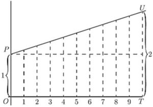
In Fig. 37, we have the corresponding illustration of the geometrical progression. Each of the successive ordinates is to be , that is, times as high as its predecessor. The steps up are not equal, because each step up is now of the ordinate at that part of the curve. If we had literally 10 steps, with for the multiplying factor, the final total would be or 2.594 times the original 1. But if only we take sufficiently large (and the corresponding sufficiently small), then the final value to which unity will grow will be 2.71828.
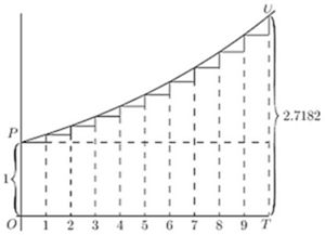
Epsilon. To this mysterious number 2.7182818 etc., the mathematicians have assigned as a symbol the Greek letter (pronounced epsilon). All schoolboys know that the Greek letter (called pi) stands for 3.141592 etc.; but how many of them know that epsilon means 2.71828? Yet it is an even more important number than !
What, then, is epsilon?
Suppose we were to let 1 grow at simple interest till it became 2; then, if at the same nominal rate of interest, and for the same time, we were to let 1 grow at true compound interest, instead of simple, it would grow to the value epsilon.
This process of growing proportionately, at every instant, to the magnitude at that instant, some people call a logarithmic rate of growing. Unit logarithmic rate of growth is that rate which in unit time will cause 1 to grow to 2.718281. It might also be called the organic rate of growing: because it is characteristic of organic growth (in certain circumstances) that the increment of the organism in a given time is proportional to the magnitude of the organism itself.
If we take 100 per cent. as the unit of rate, and any fixed period as the unit of time, then the result of letting 1 grow arithmetically at unit rate, for unit time, will be 2, while the result of letting 1 grow logarithmically at unit rate, for the same time, will be .
A little more about Epsilon. We have seen that we require to know what value is reached by the expression , when becomes indefinitely great. Arithmetically, here are tabulated a lot of values (which anybody can calculate out by the help of an ordinary table of logarithms) got by assuming and so on, up to .
It is, however, worth while to find another way of calculating this immensely important figure.
Accordingly, we will avail ourselves of the binomial theorem, and expand the expression in that well-known way.
The binomial theorem gives the rule that
Putting and , we get
Now, if we suppose to become indefinitely great, say a billion, or a billion billions, then , and , etc., will all be sensibly equal to ; and then the series becomes
By taking this rapidly convergent series to as many terms as we please, we can work out the sum to any desired point of accuracy. Here is the working for ten terms:
is incommensurable with 1, and resembles in being an interminable non-recurrent decimal.
The Exponential Series. We shall have need of yet another series.
Let us, again making use of the binomial theorem, expand the expression , which is the same as when we make indefinitely great.
But, when is made indefinitely great, this simplifies down to the following:
This series is called the exponential series.
The great reason why is regarded of importance is that possesses a property, not possessed by any other function of , that when you differentiate it its value remains unchanged; or, in other words, its differential coefficient is the same as itself. This can be instantly seen by differentiating it with respect to , thus: which is exactly the same as the original series.
Now we might have gone to work the other way, and said: Go to; let us find a function of , such that its differential coefficient is the same as itself. Or, is there any expression, involving only powers of , which is unchanged by differentiation? Accordingly; let us assume as a general expression that (in which the coefficients , etc. will have to be determined), and differentiate it.
Now, if this new expression is really to be the same as that from which it was derived, it is clear that must ; that ; that ; that , etc.
The law of change is therefore that
If, now, we take for the sake of further simplicity, we have
Differentiating it any number of times will give always the same series over again.
If, now, we take the particular case of , and evaluate the series, we shall get simply and therefore thus finally demonstrating that
[Note.—How to read exponentials. For the benefit of those who have no tutor at hand it may be of use to state that is read as "epsilon to the eksth power;" or some people read it "exponential eks." So is read "epsilon to the pee-teeth-power" or "exponential pee tee." Take some similar expressions:—Thus, is read "epsilon to the minus two power" or "exponential minus two." is read "epsilon to the minus ay-eksth" or "exponential minus ay-eks."]
Of course it follows that remains unchanged if differentiated with respect to . Also , which is equal to , will, when differentiated with respect to , be , because is a constant.
Another reason why is important is because it was made by Napier, the inventor of logarithms, the basis of his system. If is the value of , then is the logarithm, to the base , of . Or, if then
The two curves plotted in Figs. 38 and 39 represent these equations.
The points calculated are:
| 0 | 0.5 | 1 | 1.5 | 2 | |
| 1 | 1.65 | 2.71 | 4.50 | 7.39 |
| 1 | 2 | 3 | 4 | 8 | |
| 0 | 0.69 | 1.10 | 1.39 | 2.08 |
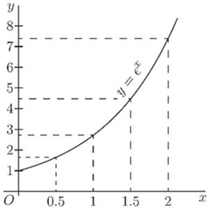
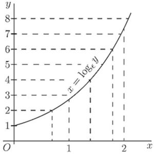
It will be seen that, though the calculations yield different points for plotting, yet the result is identical. The two equations really mean the same thing.
As many persons who use ordinary logarithms, which are calculated to base 10 instead of base , are unfamiliar with the "natural" logarithms, it may be worth while to say a word about them. The ordinary rule that adding logarithms gives the logarithm of the product still holds good; or
Also the rule of powers holds good;
But as 10 is no longer the basis, one cannot multiply by 100 or 1000 by merely adding 2 or 3 to the index. One can change the natural logarithm to the ordinary logarithm simply by multiplying it by 0.4343; or
Now let us try our hands at differentiating certain expressions that contain logarithms or exponentials.
Take the equation: First transform this into whence, since the differential of with regard to is the original function unchanged (see p. 139),
A USEFUL TABLE OF "NAPERIAN LOGARITHMS" (Also called Natural Logarithms or Hyperbolic Logarithms)
| Number | Number | ||
| 1 | 0.0000 | 6 | 1.7918 |
| 1.1 | 0.0953 | 7 | 1.9459 |
| 1.2 | 0.1823 | 8 | 2.0794 |
| 1.5 | 0.4055 | 9 | 2.1972 |
| 1.7 | 0.5306 | 10 | 2.3026 |
| 2.0 | 0.6931 | 20 | 2.9957 |
| 2.2 | 0.7885 | 50 | 3.9120 |
| 2.5 | 0.9163 | 100 | 4.6052 |
| 2.7 | 0.9933 | 200 | 5.2983 |
| 2.8 | 1.0296 | 500 | 6.2146 |
| 3.0 | 1.0986 | 1,000 | 6.9078 |
| 3.5 | 1.2528 | 2,000 | 7.6009 |
| 4.0 | 1.3863 | 5,000 | 8.5172 |
| 4.5 | 1.5041 | 10,000 | 9.2103 |
| 5.0 | 1.6094 | 20,000 | 9.9035 |
and, reverting from the inverse to the original function,
Now this is a very curious result. It may be written
Note that is a result that we could never have got by the rule for differentiating powers. That rule (page 24) is to multiply by the power, and reduce the power by 1. Thus, differentiating gave us ; and differentiating gave . But differentiating does not give us or , because is itself , and is a constant. We shall have to come back to this curious fact that differentiating gives us when we reach the chapter on integrating.
Now, try to differentiate that is we have , since the differential of remains . This gives hence, reverting to the original function (see p. 128), we get
Next try
First change to natural logarithms by multiplying by the modulus 0.4343. This gives us
The next thing is not quite so simple. Try this:
Taking the logarithm of both sides, we get
Since is a constant, we get hence, reverting to the original function.
We see that, since
We shall find that whenever we have an expression such as a function of , we always have the differential coefficient of the function of , so that we could have written at once, from ,
Let us now attempt further examples.
(1) . Let ; then .
Or thus:
(2) . Let ; then .
Or thus:
(3) .
Check by writing .
(4) .
For if and ,
Check by writing .
(5) . Let ; then .
(6) . Let ; then .
(7) .
(8) .
For if , let and .
Similarly, if ) and
(9) . and
(10)
(11) . Let .
(12) .
Try now the following exercises.
Exercises XII. (See page 260 for Answers.)
(1) Differentiate .
(2) Find the differential coefficient with respect to of the expression .
(3) If , find .
(4) Show that if .
(5) If , find .
(6) .
(7) .
(8) .
(9) .
(10) .
(11) .
(12) .
(13) It was shown by Lord Kelvin that the speed of signalling through a submarine cable depends on the value of the ratio of the external diameter of the core to the diameter of the enclosed copper wire. If this ratio is called , then the number of signals that can be sent per minute can be expressed by the formula where is a constant depending on the length and the quality of the materials. Show that if these are given, will be a maximum if .
(14) Find the maximum or minimum of
(15) Differentiate .
(16) Differentiate .
Let us return to the curve which has its successive ordinates in geometrical progression, such as that represented by the equation .
We can see, by putting , that is the initial height of . Then when
Also, we see that is the numerical value of the ratio between the height of any ordinate and that of the next preceding it. In Fig. 40, we have taken as ; each ordinate being as high as the preceding one.
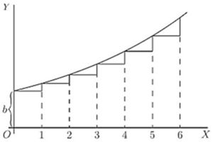
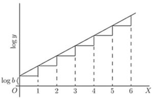
If two successive ordinates are related together thus in a constant ratio, their logarithms will have a constant difference; so that, if we should plot out a new curve, Fig. 41, with values of as ordinates, it would be a straight line sloping up by equal steps. In fact, it follows from the equation, that
Now, since is a mere number, and may be written as , it follows that and the equation takes the new form
If we were to take as a proper fraction (less than unity), the curve would obviously tend to sink downwards, as in Fig. 42, where each successive ordinate is of the height of the preceding one.
The equation is still but since is less than one, will be a negative quantity, and may be written ; so that , and now our equation for the curve takes the form
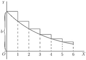
The importance of this expression is that, in the case where the independent variable is time, the equation represents the course of a great many physical processes in which something is gradually dying away. Thus, the cooling of a hot body is represented (in Newton's celebrated "law of cooling") by the equation where is the original excess of temperature of a hot body over that of its surroundings, the excess of temperature at the end of time , and is a constant-namely, the constant of decrement, depending on the amount of surface exposed by the body, and on its coefficients of conductivity and emissivity, etc.
A similar formula, is used to express the charge of an electrified body, originally having a charge , which is leaking away with a constant of decrement ; which constant depends in this case on the capacity of the body and on the resistance of the leakage-path.
Oscillations given to a flexible spring die out after a time; and the dying-out of the amplitude of the motion may be expressed in a similar way.
In fact serves as a die-away factor for all those phenomena in which the rate of decrease is proportional to the magnitude of that which is decreasing; or where, in our usual symbols, is proportional at every moment to the value that has at that moment. For we have only to inspect the curve, Fig. 42 above, to see that, at every part of it, the slope is proportional to the height ; the curve becoming flatter as grows smaller. In symbols, thus or and, differentiating, hence or, in words, the slope of the curve is downward, and proportional to and to the constant .
We should have got the same result if we had taken the equation in the form for then
But giving us as before.
The Time-constant. In the expression for the "die-away factor" , the quantity is the reciprocal of another quantity known as "the time-constant," which we may denote by the symbol . Then the die-away factor will be written ; and it will be seen, by making that the meaning of (or of ) is that this is the length of time which it takes for the original quantity (called or in the preceding instances) to die away th part—that is to 0.3678—of its original value.
The values of and are continually required in different branches of physics, and as they are given in very few sets of mathematical tables, some of the values are tabulated on p. 157 for convenience.
As an example of the use of this table, suppose there is a hot body cooling, and that at the beginning of the experiment (i.e. when ) it is hotter than the surrounding objects, and if the time-constant of its cooling is 20 minutes (that is, if it takes 20 minutes for its excess of temperature to fall to part of ), then we can calculate to what it will have fallen in any given time . For instance, let be 60 minutes. Then , and we shall have to find the value of , and then multiply the original by this. The table shows that is 0.0498. So that at the end of 60 minutes the excess of temperature will have fallen to .
| 0.00 | 1.0000 | 1.0000 | 0.0000 |
| 0.10 | 1.1052 | 0.8187 | 0.1813 |
| 0.50 | 1.6487 | 0.6065 | 0.3935 |
| 0.75 | 2.1170 | 0.4724 | 0.5276 |
| 0.90 | 2.4596 | 0.4066 | 0.5934 |
| 1.00 | 2.7183 | 0.3679 | 0.6321 |
| 1.10 | 3.0042 | 0.3329 | 0.6671 |
| 1.20 | 3.3201 | 0.3012 | 0.6988 |
| 1.25 | 3.4903 | 0.2865 | 0.7135 |
| 1.50 | 4.4817 | 0.2231 | 0.7769 |
| 1.75 | 5.755 | 0.1738 | 0.8262 |
| 2.00 | 7.389 | 0.1353 | 0.8647 |
| 2.50 | 12.182 | 0.0821 | 0.9179 |
| 3.00 | 20.086 | 0.0498 | 0.9502 |
| 3.50 | 33.115 | 0.0302 | 0.9698 |
| 4.00 | 54.598 | 0.0183 | 0.9817 |
| 4.50 | 90.017 | 0.0111 | 0.9889 |
| 5.00 | 148.41 | 0.0067 | 0.9933 |
| 5.50 | 244.69 | 0.0041 | 0.9959 |
| 6.00 | 403.43 | 0.00248 | 0.99752 |
| 7.50 | 1808.04 | 0.00055 | 0.99947 |
| 10.00 | 22026.5 | 0.000045 | 0.999955 |
(1) The strength of an electric current in a conductor at a time secs. after the application of the electromotive force producing it is given by the expression .
The time constant is .
If ; then when is very large the term becomes 1, and ; also
Its value at any time may be written: the time-constant being 0.01. This means that it takes 0.01 sec. for the variable term to fall by of its initial value .
To find the value of the current when , say, , (from table).
It follows that, after 0.001 sec., the variable term is 9.048, and the actual current is .
Similarly, at the end of 0.1 sec., the variable term is , the current being 9.9995.
(2) The intensity of a beam of light which has passed through a thickness of some transparent medium is , where is the initial intensity of the beam and is a "constant of absorption."
This constant is usually found by experiments. If it be found, for instance, that a beam of light has its intensity diminished by in passing through 10 cms. of a certain transparent medium, this means that or , and from the table one sees that very nearly; hence .
To find the thickness that will reduce the intensity to half its value, one must find the value of which satisfies the equality , or . It is found by putting this equation in its logarithmic form, namely, which gives
(3) The quantity of a radio-active substance which has not yet undergone transformation is known to be related to the initial quantity of the substance by the relation , where is a constant and the time in seconds elapsed since the transformation began.
For "Radium ," if time is expressed in seconds, experiment shows that . Find the time required for transforming half the substance. (This time is called the "mean life" of the substance.)
We have . and
Exercises XIII. (See page 260 for Answers.)
(1) Draw the curve ; where , and is given various values from 0 to 20.
(2) If a hot body cools so that in 24 minutes its excess of temperature has fallen to half the initial amount, deduce the time-constant, and find how long it will be in cooling down to 1 per cent. of the original excess.
(3) Plot the curve .
(4) The following equations give very similar curves:
Draw all three curves, taking millimetres; millimetres.
(5) Find the differential coefficient of with respect to , if
(6) For "Thorium ," the value of is 5; find the "mean life," that is, the time taken by the transformation of a quantity of "Thorium " equal to half the initial quantity in the expression being in seconds.
(7) A condenser of capacity , charged to a potential , is discharging through a resistance of 10,000 ohms. Find the potential after (a) 0.1 second; (b) 0.01 second; assuming that the fall of potential follows the rule .
(8) The charge of an electrified insulated metal sphere is reduced from 20 to 16 units in 10 minutes. Find the coefficient of leakage, if being the initial charge and being in seconds. Hence find the time taken by half the charge to leak away.
(9) The damping on a telephone line can be ascertained from the relation , where is the strength, after seconds, of a telephonic current of initial strength ; is the length of the line in kilometres, and is a constant. For the Franco-English submarine cable laid in 1910, . Find the damping at the end of the cable (40 kilometres), and the length along which is still of the original current (limiting value of very good audition).
(10) The pressure of the atmosphere at an altitude kilometres is given by being the pressure at sea-level (760 millimetres).
The pressures at 10, 20 and 50 kilometres being 199.2, 42.2, 0.32 respectively, find in each case. Using the mean value of , find the percentage error in each case.
(11) Find the minimum or maximum of .
(12) Find the minimum or maximum of .
(13) Find the minimum or maximum of .
GREEK letters being usual to denote angles, we will take as the usual letter for any variable angle the letter ("theta").
Let us consider the function
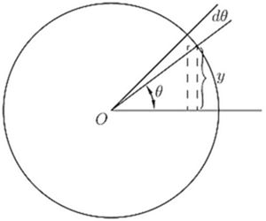
What we have to investigate is the value of ; or, in other words, if the angle varies, we have to find the relation between the increment of the sine and the increment of the angle, both increments being indefinitely small in themselves. Examine Fig. 43, wherein, if the radius of the circle is unity, the height of is the sine, and is the angle. Now, if is supposed to increase by the addition to it of the small angle —an element of angle—the height of , the sine, will be increased by a small element . The new height will be the sine of the new angle , or, stating it as an equation, and subtracting from this the first equation gives
The quantity on the right-hand side is the difference between two sines, and books on trigonometry tell us how to work this out. For they tell us that if and are two different angles,
If, then, we put for one angle, and for the other, we may write
But if we regard as indefinitely small, then in the limit we may neglect by comparison with , and may also take as being the same as . The equation then becomes:
The accompanying curves, Figs. 44 and 45, show, plotted to scale, the values of , and , for the corresponding values of .
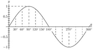
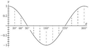
Take next the cosine.
Let .
Now .
Therefore
And it follows that
Lastly, take the tangent.
Let
Expanding, as shown in books on trigonometry,
Now remember that if is indefinitely diminished, the value of becomes identical with , and is negligibly small compared with 1, so that the expression reduces to
Collecting these results, we have:
Sometimes, in mechanical and physical questions, as, for example, in simple harmonic motion and in wave-motions, we have to deal with angles that increase in proportion to the time. Thus, if be the time of one complete period, or movement round the circle, then, since the angle all round the circle is radians, or , the amount of angle moved through in time , will be
If the frequency, or number of periods per second, be denoted by , then , and we may then write:
Then we shall have
If, now, we wish to know how the sine varies with respect to time, we must differentiate with respect, not to , but to . For this we must resort to the artifice explained in Chapter IX., p. 66, and put
Now will obviously be ; so that
Similarly, it follows that
We have seen that when is differentiated with respect to it becomes and that when is differentiated with respect to it becomes ; or, in symbols,
So we have this curious result that we have found a function such that if we differentiate it twice over, we get the same thing from which we started, but with the sign changed from + to -.
The same thing is true for the cosine; for differentiating gives us , and differentiating gives us or thus:
Sines and cosines are the only functions of which the second differential coefficient is equal (and of opposite sign to) the original function.
With what we have so far learned we can now differentiate expressions of a more complex nature.
(1) .
If is the arc whose sine is , then .
Passing now from the inverse function to the original one, we get
Now hence a rather unexpected result.
(2) .
This is the same thing as .
Let ; then ; .
(3) .
Let ; then .
(4) .
Let .
(5) .
(6) .
Let ; ; .
(7) .
Let (see p. 67). (for, if , hence )
hence .
(8) .
Exercises XIV. (See page 261 for Answers.)
(1) Differentiate the following:
(i) .
(ii) ; and .
(iii) ; and .
(2) Find the value of for which is a maximum.
(3) Differentiate .
(4) If , find .
(5) Differentiate .
(6) Differentiate .
(7) Plot the curve ; and show that the slope of the curve at is half the maximum slope.
(8) If , find .
(9) If , find the differential coefficient of with respect to .
(10) Differentiate .
(11) Differentiate the three equations of Exercises XIII. (p. 160), No. 4, and compare their differential coefficients, as to whether they are equal, or nearly equal, for very small values of , or for very large values of , or for values of in the neighbourhood of .
(12) Differentiate the following:
(i) .
(ii) .
(iii) .
(iv) .
(v) .
(13) Differentiate .
(14) Differentiate .
(15) Find the maximum or minimum of .
WE sometimes come across quantities that are functions of more than one independent variable. Thus, we may find a case where depends on two other variable quantities, one of which we will call and the other . In symbols
Take the simplest concrete case.
Let .
What are we to do? If we were to treat as a constant, and differentiate with respect to , we should get or if we treat as a constant, and differentiate with respect to , we should have:
The little letters here put as subscripts are to show which quantity has been taken as constant in the operation.
Another way of indicating that the differentiation has been performed only partially, that is, has been performed only with respect to one of the independent variables, is to write the differential coefficients with Greek deltas, like , instead of little . In this way
If we put in these values for and respectively, we shall have
But, if you think of it, you will observe that the total variation of depends on both these things at the same time. That is to say, if both are varying, the real ought to be written and this is called a total differential. In some books it is written .
Example (1). Find the partial differential coefficients of the expression . The answers are:
The first is obtained by supposing constant, the second is obtained by supposing constant; then
Example (2). Let . Then, treating first and then as constant, we get in the usual way so that .
Example (3). A cone having height and radius of base has volume . If its height remains constant, while changes, the ratio of change of volume, with respect to radius, is different from ratio of change of volume with respect to height which would occur if the height were varied and the radius kept constant, for
The variation when both the radius and the height change is given by .
Example (4). In the following example and denote two arbitrary functions of any form whatsoever. For example, they may be sine-functions, or exponentials, or mere algebraic functions of the two independent variables, and . This being understood, let us take the expression or, where
Then (where the figure 1 is simply the coefficient of in and ); and
Also and whence
This differential equation is of immense importance in mathematical physics.
Example (5). Let us take up again Exercise IX., p. 107, No. 4.
Let and be the length of two of the portions of the string. The third is , and the area of the triangle is , where is the half perimeter, 15, so that , where
Clearly is maximum when is maximum. For a maximum (clearly it will not be a minimum in this case), one must have simultaneously that is,
An immediate solution is .
If we now introduce this condition in the value of , we find For maximum or minimum, , which gives or .
Clearly gives minimum area; gives the maximum, for , which is +30 for and -30 for .
Example (6). Find the dimensions of an ordinary railway coal truck with rectangular ends, so that, for a given volume the area of sides and floor together is as small as possible.
The truck is a rectangular box open at the top. Let be the length and be the width; then the depth is . The surface area is
For minimum (clearly it won't be a maximum here),
Here also, an immediate solution is , so that , for minimum, and
Exercises XV. (See page 263 for Answers.)
(1) Differentiate the expression with respect to alone, and with respect to alone.
(2) Find the partial differential coefficients with respect to and , of the expression
(3) Let .
Find the value of . Also find the value of .
(4) Find the total differential of .
(5) Find the total differential of ; of ; and of .
(6) Verify that the sum of three quantities , , , whose product is a constant , is maximum when these three quantities are equal.
(7) Find the maximum or minimum of the function
(8) The post-office regulations state that no parcel is to be of such a size that its length plus its girth exceeds 6 feet. What is the greatest volume that can be sent by post (a) in the case of a package of rectangular cross section; (b) in the case of a package of circular cross section.
(9) Divide into 3 parts such that the continued product of their sines may be a maximum or minimum.
(10) Find the maximum or minimum of .
(11) Find maximum and minimum of
(12) A telpherage bucket of given capacity has the shape of a horizontal isosceles triangular prism with the apex underneath, and the opposite face open. Find its dimensions in order that the least amount of iron sheet may be used in its construction.
THE great secret has already been revealed that this mysterious symbol , which is after all only a long , merely means "the sum of," or "the sum of all such quantities as." It therefore resembles that other symbol (the Greek Sigma), which is also a sign of summation. There is this difference, however, in the practice of mathematical men as to the use of these signs, that while is generally used to indicate the sum of a number of finite quantities, the integral sign is generally used to indicate the summing up of a vast number of small quantities of indefinitely minute magnitude, mere elements in fact, that go to make up the total required. Thus , and .
Any one can understand how the whole of anything can be conceived of as made up of a lot of little bits; and the smaller the bits the more of them there will be. Thus, a line one inch long may be conceived as made up of 10 pieces, each of an inch long; or of 100 parts, each part being of an inch long; or of parts, each of which is of an inch long; or, pushing the thought to the limits of conceivability, it may be regarded as made up of an infinite number of elements each of which is infinitesimally small.
Yes, you will say, but what is the use of thinking of anything that way? Why not think of it straight off, as a whole? The simple reason is that there are a vast number of cases in which one cannot calculate the bigness of the thing as a whole without reckoning up the sum of a lot of small parts. The process of "integrating" is to enable us to calculate totals that otherwise we should be unable to estimate directly.
Let us first take one or two simple cases to familiarize ourselves with this notion of summing up a lot of separate parts.
Consider the series:
Here each member of the series is formed by taking it half the value of the preceding. What is the value of the total if we could go on to an infinite number of terms? Every schoolboy knows that the answer is 2. Think of it, if you like, as a line.

Begin with one inch; add a half inch, add a quarter; add an eighth; and so on. If at any point of the operation we stop, there will still be a piece wanting to make up the whole 2 inches; and the piece wanting will always be the same size as the last piece added. Thus, if after having put together , and , we stop, there will be wanting. If we go on till we have added , there will still be wanting. The remainder needed will always be equal to the last term added. By an infinite number of operations only should we reach the actual 2 inches. Practically we should reach it when we got to pieces so small that they could not be drawn-that would be after about 10 terms, for the eleventh term is . If we want to go so far that not even a Whitworth's measuring machine would detect it, we should merely have to go to about 20 terms. A microscope would not show even the term! So the infinite number of operations is no such dreadful thing after all. The integral is simply the whole lot. But, as we shall see, there are cases in which the integral calculus enables us to get at the exact total that there would be as the result of an infinite number of operations. In such cases the integral calculus gives us a rapid and easy way of getting at a result that would otherwise require an interminable lot of elaborate working out. So we had best lose no time in learning how to integrate.
Let us make a little preliminary enquiry about the slopes of curves. For we have seen that differentiating a curve means finding an expression for its slope (or for its slopes at different points). Can we perform the reverse process of reconstructing the whole curve if the slope (or slopes) are prescribed for us?
Go back to case (2) on p. 82. Here we have the simplest of curves, a sloping line with the equation
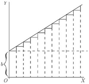
We know that here represents the initial height of when , and that , which is the same as , is the "slope" of the line. The line has a constant slope. All along it the elementary triangles have the same proportion between height and base. Suppose we were to take the 's, and 's of finite magnitude, so that 's made up one inch, then there would be ten little triangles like

Now, suppose that we were ordered to reconstruct the "curve," starting merely from the information that . What could we do? Still taking the little 's as of finite size, we could draw 10 of them, all with the same slope, and then put them together, end to end, like this:
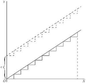
And, as the slope is the same for all, they would join to make, as in Fig. 48, a sloping line sloping with the correct slope . And whether we take the 's and 's as finite or infinitely small, as they are all alike, clearly , if we reckon as the total of all the 's, and as the total of all the 's. But whereabouts are we to put this sloping line? Are we to start at the origin , or higher up? As the only information we have is as to the slope, we are without any instructions as to the particular height above ; in fact the initial height is undetermined. The slope will be the same, whatever the initial height. Let us therefore make a shot at what may be wanted, and start the sloping line at a height above . That is, we have the equation
It becomes evident now that in this case the added constant means the particular value that has when .
Now let us take a harder case, that of a line, the slope of which is not constant, but turns up more and more. Let us assume that the upward slope gets greater and greater in proportion as grows. In symbols this is: Or, to give a concrete case, take , so that
Then we had best begin by calculating a few of the values of the slope at different values of , and also draw little diagrams of them.
When
Now try to put the pieces together, setting each so that the middle of its base is the proper distance to the right, and so that they fit together at the corners; thus (Fig. 49). The result is, of course, not a smooth curve: but it is an approximation to one. If we had taken bits half as long, and twice as numerous, like Fig. 50, we should have a better approximation. But for a perfect curve we ought to take each and its corresponding infinitesimally small, and infinitely numerous.
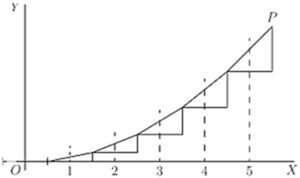
Then, how much ought the value of any to be? Clearly, at any point of the curve, the value of will be the sum of all the little 's from 0 up to that level, that is to say, . And as each is equal to , it follows that the whole will be equal to the sum of all such bits as , or, as we should write it, .
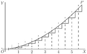
Now if had been constant, would have been the same as , or . But began by being 0, and increases to the particular value of at the point , so that its average value from 0 to that point is . Hence ; or .
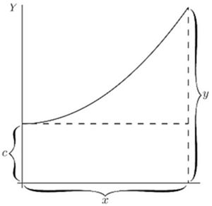
But, as in the previous case, this requires the addition of an undetermined constant , because we have not been told at what height above the origin the curve will begin, when . So we write, as the equation of the curve drawn in Fig. 51,
Exercises XVI. (See page 264 for Answers.)
(1) Find the ultimate sum of etc.
(2) Show that the series etc., is convergent, and find its sum to 8 terms.
(3) If etc., find .
(4) Following a reasoning similar to that explained in this chapter, find ,
(5) If , find .
DIFFERENTIATING is the process by which when is given us (as a function of ), we can find .
Like every other mathematical operation, the process of differentiation may be reversed; thus, if differentiating gives us ; if one begins with one would say that reversing the process would yield . But here comes in a curious point. We should get if we had begun with any of the following: , or , or , or with any added constant. So it is clear that in working backwards from to , one must make provision for the possibility of there being an added constant, the value of which will be undetermined until ascertained in some other way. So, if differentiating yields , going backwards from will give us ; where stands for the yet undetermined possible constant.
Clearly, in dealing with powers of , the rule for working backwards will be: Increase the power by 1, then divide by that increased power, and add the undetermined constant.
So, in the case where working backwards, we get
If differentiating the equation gives us it is a matter of common sense that beginning with and reversing the process, will give us So, when we are dealing with a multiplying constant, we must simply put the constant as a multiplier of the result of the integration.
Thus, if , the reverse process gives us .
But this is incomplete. For we must remember that if we had started with where is any constant quantity whatever, we should equally have found
So, therefore, when we reverse the process we must always remember to add on this undetermined constant, even if we do not yet know what its value will be.
This process, the reverse of differentiating, is called integrating; for it consists in finding the value of the whole quantity when you are given only an expression for or for . Hitherto we have as much as possible kept and together as a differential coefficient: henceforth we shall more often have to separate them.
If we begin with a simple case,
We may write this, if we like, as
Now this is a "differential equation" which informs us that an element of is equal to the corresponding element of multiplied by . Now, what we want is the integral; therefore, write down with the proper symbol the instructions to integrate both sides, thus:
[Note as to reading integrals: the above would be read thus:
"Integral dee-wy equals integral eks-squared dee-eks."]
We haven't yet integrated: we have only written down instructions to integrate—if we can. Let us try. Plenty of other fools can do it-why not we also? The left-hand side is simplicity itself. The sum of all the bits of is the same thing as itself. So we may at once put:
But when we come to the right-hand side of the equation we must remember that what we have got to sum up together is not all the 's, but all such terms as ; and this will not be the same as , because is not a constant. For some of the 's will be multiplied by big values of , and some will be multiplied by small values of , according to what happens to be. So we must bethink ourselves as to what we know about this process of integration being the reverse of differentiation. Now, our rule for this reversed process—see p. 189 ante—when dealing with is "increase the power by one, and divide by the same number as this increased power." That is to say, will be changed to . Put this into the equation; but don't forget to add the "constant of integration" at the end. So we get:
Footnote: [You may ask, what has become of the little at the end? Well, remember that it was really part of the differential coefficient, and when changed over to the right-hand side, as in the , serves as a reminder that is the independent variable with respect to which the operation is to be effected; and, as the result of the product being totalled up, the power of has increased by one. You will soon become familiar with all this.]
You have actually performed the integration. How easy!
Let us try another simple case.
Let where is any constant multiplier. Well, we found when differentiating (see p. 27) that any constant factor in the value of reappeared unchanged in the value of . In the reversed process of integrating, it will therefore also reappear in the value of . So we may go to work as before, thus
So that is done. How easy!
We begin to realize now that integrating is a process of finding our way back, as compared with differentiating. If ever, during differentiating, we have found any particular expression-in this example —we can find our way back to the from which it was derived. The contrast between the two processes may be illustrated by the following remark due to a well-known teacher. If a stranger were set down in Trafalgar Square, and told to find his way to Euston Station, he might find the task hopeless. But if he had previously been personally conducted from Euston Station to Trafalgar Square, it would be comparatively easy to him to find his way back to Euston Station.
Let then
There is no reason why we should not integrate each term separately: for, as may be seen on p. 34, we found that when we differentiated the sum of two separate functions, the differential coefficient was simply the sum of the two separate differentiations. So, when we work backwards, integrating, the integration will be simply the sum of the two separate integrations.
Our instructions will then be:
If either of the terms had been a negative quantity, the corresponding term in the integral would have also been negative. So that differences are as readily dealt with as sums.
Suppose there is in the expression to be integrated a constant term—such as this:
This is laughably easy. For you have only to remember that when you differentiated the expression , the result was . Hence, when you work the other way and integrate, the constant reappears multiplied by . So we get
Here are a lot of examples on which to try your newly acquired powers.
(1) Given . Find Ans. .
(2) Find . It is or or .
(3) Given . Find . Ans. .
(4) . Find . and
(5) Integrate . Ans. .
All these are easy enough. Let us try another case.
Let .
Proceeding as before, we will write
Well, but what is the integral of ?
If you look back amongst the results of differentiating and and , etc., you will find we never got from any one of them as the value of . We got from ; we got from ; we got 1 from (that is, from itself); but we did not get from , for two very good reasons. First, is simply , and is a constant, and could not have a differential coefficient. Secondly, even if it could be differentiated, its differential coefficient (got by slavishly following the usual rule) would be , and that multiplication by zero gives it zero value! Therefore when we now come to try to integrate , we see that it does not come in anywhere in the powers of that are given by the rule: It is an exceptional case.
Well; but try again. Look through all the various differentials obtained from various functions of , and try to find amongst them . A sufficient search will show that we actually did get as the result of differentiating the function (see p. 145).
Then, of course, since we know that differentiating gives us , we know that, by reversing the process, integrating will give us . But we must not forget the constant factor that was given, nor must we omit to add the undetermined constant of integration. This then gives us as the solution to the present problem,
N.B.—Here note this very remarkable fact, that we could not have integrated in the above case if we had not happened to know the corresponding differentiation. If no one had found out that differentiating gave , we should have been utterly stuck by the problem how to integrate . Indeed it should be frankly admitted that this is one of the curious features of the integral calculus:—that you can't integrate anything before the reverse process of differentiating something else has yielded that expression which you want to integrate. No one, even to-day, is able to find the general integral of the expression, because has never yet been found to result from differentiating anything else.
Another simple case.
Find .
On looking at the function to be integrated, you remark that it is the product of two different functions of . You could, you think, integrate by itself, or by itself. Of course you could. But what to do with a product? None of the differentiations you have learned have yielded you for the differential coefficient a product like this. Failing such, the simplest thing is to multiply up the two functions, and then integrate. This gives us And this is the same as And performing the integrations, we get
Now that we know that integration is the reverse of differentiation, we may at once look up the differential coefficients we already know, and see from what functions they were derived. This gives us the following integrals ready made: (for if ).
Also we may deduce the following: (for if ). (for if ; hence to get one must differentiate ).
Try also ; a little dodge will simplify matters: and
See also the Table of Standard Forms on pp. 249-251. You should make such a table for yourself, putting in it only the general functions which you have successfully differentiated and integrated. See to it that it grows steadily!
In many cases it is necessary to integrate some expression for two or more variables contained in it; and in that case the sign of integration appears more than once. Thus, means that some function of the variables and has to be integrated for each. It does not matter in which order they are done. Thus, take the function . Integrating it with respect to gives us:
Now, integrate this with respect to : to which of course a constant is to be added. If we had reversed the order of the operations, the result would have been the same.
In dealing with areas of surfaces and of solids, we have often to integrate both for length and breadth, and thus have integrals of the form where is some property that depends, at each point, on and on . This would then be called a surface-integral. It indicates that the value of all such elements as (that is to say, of the value of over a little rectangle long and broad) has to be summed up over the whole length and whole breadth.
Similarly in the case of solids, where we deal with three dimensions. Consider any element of volume, the small cube whose dimensions are . If the figure of the solid be expressed by the function , then the whole solid will have the volume-integral, Naturally, such integrations have to be taken between appropriate limits in each dimension; and the integration cannot be performed unless one knows in what way the boundaries of the surface depend on , , and . If the limits for are from to , those for from to , and those for from to , then clearly we have
Footnote: See p. 206 for integration between limits.
There are of course plenty of complicated and difficult cases; but, in general, it is quite easy to see the significance of the symbols where they are intended to indicate that a certain integration has to be performed over a given surface, or throughout a given solid space.
Exercises XVII. (See p. 264 for the Answers.)
(1) Find when .
(2) Find .
(3) Find .
(4) Find .
(5) Integrate .
(6) Find .
(7) If ; find .
(8) Find .
(9) Find .
(10) Find .
(11) Find .
(12) Find .
(13) Find .
(14) Find .
(15) Find .
(16) Find .
(17) Find .
(18) Find .
ONE use of the integral calculus is to enable us to ascertain the values of areas bounded by curves.
Let us try to get at the subject bit by bit.
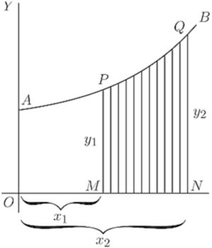
Let (Fig. 52) be a curve, the equation to which is known. That is, in this curve is some known function of . Think of a piece of the curve from the point to the point .
Let a perpendicular be dropped from , and another from the point . Then call and , and the ordinates and . We have thus marked out the area that lies beneath the piece . The problem is, how can we calculate the value of this area?
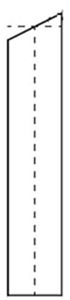
The secret of solving this problem is to conceive the area as being divided up into a lot of narrow strips, each of them being of the width . The smaller we take , the more of them there will be between and . Now, the whole area is clearly equal to the sum of the areas of all such strips. Our business will then be to discover an expression for the area of any one narrow strip, and to integrate it so as to add together all the strips. Now think of any one of the strips. will be like this: being bounded between two vertical sides, with a flat bottom , and with a slightly curved sloping top. Suppose we take its average height as being ; then, as its width is , its area will be . And seeing that we may take the width as narrow as we please, if we only take it narrow enough its average height will be the same as the height at the middle of it. Now let us call the unknown value of the whole area , meaning surface. The area of one strip will be simply a bit of the whole area, and may therefore be called . So we may write If then we add up all the strips, we get
So then our finding depends on whether we can integrate for the particular case, when we know what the value of is as a function of .
For instance, if you were told that for the particular curve in question , no doubt you could put that value into the expression and say: then I must find .
That is all very well; but a little thought will show you that something more must be done. Because the area we are trying to find is not the area under the whole length of the curve, but only the area limited on the left by , and on the right by , it follows that we must do something to define our area between those 'limits.'
This introduces us to a new notion, namely that of integrating between limits. We suppose to vary, and for the present purpose we do not require any value of below (that is ), nor any value of above (that is ). When an integral is to be thus defined between two limits, we call the lower of the two values the inferior limit, and the upper value the superior limit. Any integral so limited we designate as a definite integral, by way of distinguishing it from a general integral to which no limits are assigned.
In the symbols which give instructions to integrate, the limits are marked by putting them at the top and bottom respectively of the sign of integration. Thus the instruction will be read: find the integral of between the inferior limit and the superior limit .
Sometimes the thing is written more simply Well, but how do you find an integral between limits, when you have got these instructions?
Look again at Fig. 52 (p. 204). Suppose we could find the area under the larger piece of curve from to , that is from to , naming the area . Then, suppose we could find the area under the smaller piece from to , that is from to , namely the area . If then we were to subtract the smaller area from the larger, we should have left as a remainder the area , which is what we want. Here we have the clue as to what to do; the definite integral between the two limits is the difference between the integral worked out for the superior limit and the integral worked out for the lower limit.
Let us then go ahead. First, find the general integral thus: and, as is the equation to the curve (Fig. 52), is the general integral which we must find.
Doing the integration in question by the rule (p. 193), we get and this will be the whole area from 0 up to any value of that we may assign.
Therefore, the larger area up to the superior limit will be and the smaller area up to the inferior limit will be
Now, subtract the smaller from the larger, and we get for the area the value,
This is the answer we wanted. Let us give some numerical values. Suppose , and and . Then the area is equal to
Let us here put down a symbolic way of stating what we have ascertained about limits: where is the integrated value of corresponding to , and that corresponding to .
All integration between limits requires the difference between two values to be thus found. Also note that, in making the subtraction the added constant has disappeared.
(1) To familiarize ourselves with the process, let us take a case of which we know the answer beforehand. Let us find the area of the triangle (Fig. 53), which has base and height . We know beforehand, from obvious mensuration, that the answer will come 24.
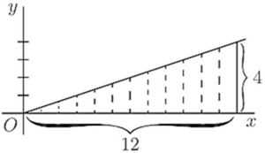
Now, here we have as the "curve" a sloping line for which the equation is
The area in question will be
Integrating (p. 192), and putting down the value of the general integral in square brackets with the limits marked above and below, we get
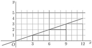
Let us satisfy ourselves about this rather surprising dodge of calculation, by testing it on a simple example. Get some squared paper, preferably some that is ruled in little squares of one-eighth inch or one-tenth inch each way. On this squared paper plot out the graph of the equation,
The values to be plotted will be:
| 0 | 3 | 6 | 9 | 12 | |
| 0 | 1 | 2 | 3 | 4 |
The plot is given in Fig. 54.
Now reckon out the area beneath the curve by counting the little squares below the line, from as far as on the right. There are 18 whole squares and four triangles, each of which has an area equal to squares; or, in total, 24 squares. Hence 24 is the numerical value of the integral of between the lower limit of and the higher limit of .
As a further exercise, show that the value of the same integral between the limits of and is 36.
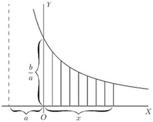
(2) Find the area, between limits and , of the curve .
N.B.—Notice that in dealing with definite integrals the constant always disappears by subtraction.
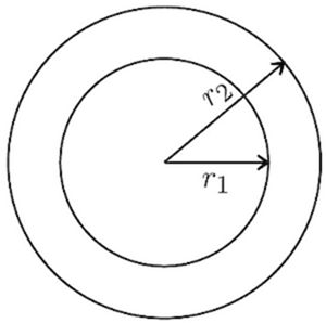
Let it be noted that this process of subtracting one part from a larger to find the difference is really a common practice. How do you find the area of a plane ring (Fig. 56), the outer radius of which is and the inner radius is ? You know from mensuration that the area of the outer circle is ; then you find the area of the inner circle, ; then you subtract the latter from the former, and find area of ring ; which may be written mean circumference of ring × width of ring.
(3) Here's another case - that of the die-away curve (p. 153). Find the area between and , of the curve (Fig. 57) whose equation is
The integration (p. 198) gives
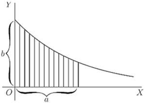
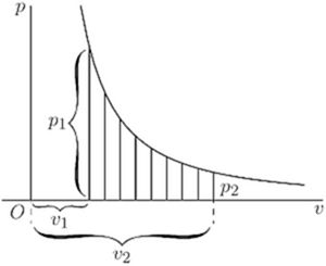
(4) Another example is afforded by the adiabatic curve of a perfect gas, the equation to which is , where stands for pressure, for volume, and is of the value 1.42 (Fig. 58).
Find the area under the curve (which is proportional to the work done in suddenly compressing the gas) from volume to volume .
Here we have
Prove the ordinary mensuration formula, that the area of a circle whose radius is , is equal to .
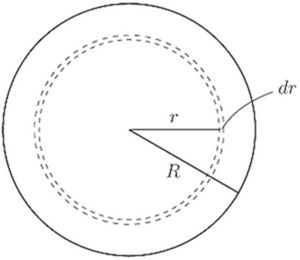
Consider an elementary zone or annulus of the surface (Fig. 59), of breadth , situated at a distance from the centre. We may consider the entire surface as consisting of such narrow zones, and the whole area will simply be the integral of all such elementary zones from centre to margin, that is, integrated from to .
We have therefore to find an expression for the elementary area of the narrow zone. Think of it as a strip of breadth , and of a length that is the periphery of the circle of radius , that is, a length of . Then we have, as the area of the narrow zone,
Hence the area of the whole circle will be:
Now, the general integral of is . Therefore,
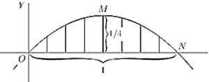
Let us find the mean ordinate of the positive part of the curve , which is shown in Fig. 60. To find the mean ordinate, we shall have to find the area of the piece , and then divide it by the length of the base . But before we can find the area we must ascertain the length of the base, so as to know up to what limit we are to integrate. At the ordinate has zero value; therefore, we must look at the equation and see what value of will make . Now, clearly, if is will also be 0, the curve passing through the origin ; but also, if ; so that gives us the position of the point .
Then the area wanted is
But the base length is 1.
Therefore, the average ordinate of the curve .
[N.B.—It will be a pretty and simple exercise in maxima and minima to find by differentiation what is the height of the maximum ordinate. It must be greater than the average.]
The mean ordinate of any curve, over a range from to , is given by the expression,
One can also find in the same way the surface area of a solid of revolution.
The curve is revolving about the axis of . Find the area of the surface generated by the curve between and .
A point on the curve, the ordinate of which is , describes a circumference of length , and a narrow belt of the surface, of width , corresponding to this point, has for area . The total area is
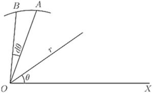
When the equation of the boundary of an area is given as a function of the distance of a point of it from a fixed point (see Fig. 61) called the pole, and of the angle which makes with the positive horizontal direction , the process just explained can be applied just as easily, with a small modification. Instead of a strip of area, we consider a small triangle , the angle at being , and we find the sum of all the little triangles making up the required area.
The area of such a small triangle is approximately or ; hence the portion of the area included between the curve and two positions of corresponding to the angles and is given by
(1) Find the area of the sector of 1 radian in a circumference of radius inches.
The polar equation of the circumference is evidently . The area is
(2) Find the area of the first quadrant of the curve (known as "Pascal's Snail"), the polar equation of which is .
What we have done with the area of a little strip of a surface, we can, of course, just as easily do with the volume of a little strip of a solid. We can add up all the little strips that make up the total solid, and find its volume, just as we have added up all the small little bits that made up an area to find the final area of the figure operated upon.
(1) Find the volume of a sphere of radius .
A thin spherical shell has for volume (see Fig. 59, p. 214); summing up all the concentric shells which make up the sphere, we have
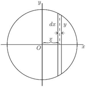
We can also proceed as follows: a slice of the sphere, of thickness , has for volume (see Fig. 62). Also and are related by the expression
(2) Find the volume of the solid generated by the revolution of the curve about the axis of , between and .
The volume of a strip of the solid is .
Hence
In certain branches of physics, particularly in the study of alternating electric currents, it is necessary to be able to calculate the quadratic mean of a variable quantity. By "quadratic mean" is denoted the square root of the mean of the squares of all the values between the limits considered. Other names for the quadratic mean of any quantity are its "virtual" value, or its "R.M.S." (meaning root-mean-square) value. The French term is valeur efficace. If is the function under consideration, and the quadratic mean is to be taken between the limits of and ; then the quadratic mean is expressed as
(1) To find the quadratic mean of the function (Fig. 63).
Here the integral is , which is . Dividing by and taking the square root, we have
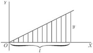
Here the arithmetical mean is ; and the ratio of quadratic to arithmetical mean (this ratio is called the form-factor) is .
(2) To find the quadratic mean of the function .
The integral is , that is .
Hence
(3) To find the quadratic mean of the function .
The integral is , that is , which is .
Hence the quadratic mean is .
Exercises XVIII. (See p. 265 for Answers.)
(1) Find the area of the curve between and , and the mean ordinates between these limits.
(2) Find the area of the parabola between and . Show that it is two-thirds of the rectangle of the limiting ordinate and of its abscissa.
(3) Find the area of the positive portion of a sine curve and the mean ordinate.
(4) Find the area of the positive portion of the curve , and find the mean ordinate.
(5) Find the area included between the two branches of the curve from to , also the area of the positive portion of the lower branch of the curve (see Fig. 30, p. 106).
(6) Find the volume of a cone of radius of base , and of height .
(7) Find the area of the curve between and .
(8) Find the volume generated by the curve , as it revolves about the axis of , between and .
(9) Find the volume generated by a sine curve revolving about the axis of . Find also the area of its surface.
(10) Find the area of the portion of the curve included between and . Find the mean ordinate between these limits.
(11) Show that the quadratic mean of the function , between the limits of 0 and radians, is . Find also the arithmetical mean of the same function between the same limits; and show that the form-factor is .
(12) Find the arithmetical and quadratic means of the function , from to .
(13) Find the quadratic mean and the arithmetical mean of the function .
(14) A certain curve has the equation . Find the area included between the curve and the axis of , from the ordinate at to the ordinate at . Find also the height of the mean ordinate of the curve between these points.
(15) Show that the radius of a circle, the area of which is twice the area of a polar diagram, is equal to the quadratic mean of all the values of for that polar diagram.
(16) Find the volume generated by the curve rotating about the axis of .
Dodges. A great part of the labour of integrating things consists in licking them into some shape that can be integrated. The books-and by this is meant the serious books-on the Integral Calculus are full of plans and methods and dodges and artifices for this kind of work. The following are a few of them.
Integration by Parts. This name is given to a dodge, the formula for which is
It is useful in some cases that you can't tackle directly, for it shows that if in any case can be found, then can also be found. The formula can be deduced as follows. From p. 37, we have, which may be written which by direct integration gives the above expression.
(1) Find .
Write , and for write . We shall then have , while .
Putting these into the formula, we get
(2) Find .
Write then and
(3) Try .
Hence and
(4) Find .
Write then
Now find , integrating by parts (as in Example 1 above):
Hence
(5) Find .
Write then (see Chap. IX., p. 66). and ; so that
Here we may use a little dodge, for we can write
Adding these two last equations, we get rid of , and we have
Do you remember meeting ? it is got by differentiating (see p. 168); hence its integral is , and so
You can try now some exercises by yourself; you will find some at the end of this chapter.
Substitution. This is the same dodge as explained in Chap. IX., p. 66. Let us illustrate its application to integration by a few examples.
(1) .
Let replace
(2) .
Let so that
is the result of differentiating . Hence the integral is .
(3) .
Let then the integral becomes ; but is the result of differentiating .
Hence one has finally for the value of the given integral.
Formulæ of Reduction are special forms applicable chiefly to binomial and trigonometrical expressions that have to be integrated, and have to be reduced into some form of which the integral is known.
Rationalization, and Factorization of Denominator are dodges applicable in special cases, but they do not admit of any short or general explanation. Much practice is needed to become familiar with these preparatory processes.
The following example shows how the process of splitting into partial fractions, which we learned in Chap. XIII., p. 118, can be made use of in integration.
Take again ; if we split into partial fractions, this becomes (see p. 230): Notice that the same integral can be expressed sometimes in more than one way (which are equivalent to one another).
Pitfalls. A beginner is liable to overlook certain points that a practised hand would avoid; such as the use of factors that are equivalent to either zero or infinity, and the occurrence of indeterminate quantities such as . There is no golden rule that will meet every possible case. Nothing but practice and intelligent care will avail. An example of a pitfall which had to be circumvented arose in Chap. XVIII., p. 189, when we came to the problem of integrating .
Triumphs. By triumphs must be understood the successes with which the calculus has been applied to the solution of problems otherwise intractable. Often in the consideration of physical relations one is able to build up an expression for the law governing the interaction of the parts or of the forces that govern them, such expression being naturally in the form of a differential equation, that is an equation containing differential coefficients with or without other algebraic quantities. And when such a differential equation has been found, one can get no further until it has been integrated. Generally it is much easier to state the appropriate differential equation than to solve it: the real trouble begins then only when one wants to integrate, unless indeed the equation is seen to possess some standard form of which the integral is known, and then the triumph is easy. The equation which results from integrating a differential equation is called its "solution"; and it is quite astonishing how in many cases the solution looks as if it had no relation to the differential equation of which it is the integrated form. The solution often seems as different from the original expression as a butterfly does from the caterpillar that it was. Who would have supposed that such an innocent thing as could blossom out into yet the latter is the solution of the former.
Footnote: This means that the actual result of solving it is called its "solution." But many mathematicians would say, with Professor Forsyth, "every differential equation is considered as solved when the value of the dependent variable is expressed as a function of the independent variable by means either of known functions, or of integrals, whether the integrations in the latter can or cannot be expressed in terms of functions already known."
As a last example, let us work out the above together.
By partial fractions,
Not a very difficult metamorphosis!
There are whole treatises, such as Boole's Differential Equations, devoted to the subject of thus finding the "solutions" for different original forms.
Exercises XIX. (See p. 266 for Answers.)
(1) Find .
(2) Find .
(3) Find .
(4) Find .
(5) Find .
(6) Find .
(7) Find .
(8) Find .
(9) Find .
(10) Find .
(11) Find .
(12) Find .
(13) Find .
(14) Find .
IN this chapter we go to work finding solutions to some important differential equations, using for this purpose the processes shown in the preceding chapters.
The beginner, who now knows how easy most of those processes are in themselves, will here begin to realize that integration is an art. As in all arts, so in this, facility can be acquired only by diligent and regular practice. He who would attain that facility must work out examples, and more examples, and yet more examples, such as are found abundantly in all the regular treatises on the Calculus. Our purpose here must be to afford the briefest introduction to serious work.
Example 1. Find the solution of the differential equation
Transposing we have
Now the mere inspection of this relation tells us that we have got to do with a case in which is proportional to . If we think of the curve which will represent as a function of , it will be such that its slope at any point will be proportional to the ordinate at that point, and will be a negative slope if is positive. So obviously the curve will be a die-away curve (p. 153), and the solution will contain as a factor. But, without presuming on this bit of sagacity, let us go to work.
As both and occur in the equation and on opposite sides, we can do nothing until we get both and to one side, and to the other. To do this, we must split our usually inseparable companions and from one another.
Having done the deed, we now can see that both sides have got into a shape that is integrable, because we recognize , or , as a differential that we have met with (p. 143) when differentiating logarithms. So we may at once write down the instructions to integrate, and doing the two integrations, we have: where is the yet undetermined constant of integration. Then, delogarizing, we get: which is the solution required. Now, this solution looks quite unlike the original differential equation from which it was constructed: yet to an expert mathematician they both convey the same information as to the way in which depends on .
Footnote: We may write down any form of constant as the "constant of integration," and the form is adopted here by preference, because the other terms in this line of equation are, or are treated as logarithms; and it saves complications afterward if the added constant be of the same kind.
Now, as to the , its meaning depends on the initial value of . For if we put in order to see what value then has, we find that this makes ; and as we see that is nothing else than the particular value of at starting. This we may call , and so write the solution as
Footnote: Compare what was said about the "constant of integration," with reference to Fig. 48 on p. 184, and Fig. 51 on p. 187.
Let us take as an example to solve where is a constant. Again, inspecting the equation will suggest, (1) that somehow or other will come into the solution, and (2) that if at any part of the curve becomes either a maximum or a minimum, so that , then will have the value . But let us go to work as before, separating the differentials and trying to transform the thing into some integrable shape.
Now we have done our best to get nothing but and on one side, and nothing but on the other. But is the result on the left side integrable?
It is of the same form as the result on p. 145; so, writing the instructions to integrate, we have: and, doing the integration, and adding the appropriate constant, and finally, which is the solution.
If the condition is laid down that when we can find ; for then the exponential becomes ; and we have
Putting in this value, the solution becomes
But further, if grows indefinitely, will grow to a maximum; for when , the exponential , giving . Substituting this, we get finally
This result is also of importance in physical science.
Example 3.
Let
We shall find this much less tractable than the preceding. First divide through by .
Now, as it stands, the left side is not integrable. But it can be made so by the artifice - and this is where skill and practice suggest a plan-of multiplying all the terms by , giving us: which is the same as and this being a perfect differential may be integrated thus:-since, if ,
The last term is obviously a term which will die out as increases, and may be omitted. The trouble now comes in to find the integral that appears as a factor. To tackle this we resort to the device (see p. 224) of integration by parts, the general formula for which is . For this purpose write
We shall then have
Inserting these, the integral in question becomes:
The last integral is still irreducible. To evade the difficulty, repeat the integration by parts of the left side, but treating it in the reverse way by writing:
Inserting these, we get
Noting that the final intractable integral in [C] is the same as that in , we may eliminate it, by multiplying by , and multiplying [c] by , and adding them.
The result, when cleared down, is:
Inserting this value in , we get
To simplify still further, let us imagine an angle such that .
Then and
Substituting these, we get: which may be written which is the solution desired.
This is indeed none other than the equation of an alternating electric current, where represents the amplitude of the electromotive force, the frequency, the resistance, the coefficient of self-induction of the circuit, and is an angle of lag.
Suppose that .
We could integrate this expression directly, if were a function of only, and a function of only; but, if both and are functions that depend on both and , how are we to integrate it? Is it itself an exact differential? That is: have and each been formed by partial differentiation from some common function , or not? If they have, then And if such a common function exists, then is an exact differential (compare p. 172).
Now the test of the matter is this. If the expression is an exact differential, it must be true that which is necessarily true.
Take as an illustration the equation
Is this an exact differential or not? Apply the test. which do not agree. Therefore, it is not an exact differential, and the two functions and have not come from a common original function.
It is possible in such cases to discover, however, an integrating factor, that is to say, a factor such that if both are multiplied by this factor, the expression will become an exact differential. There is no one rule for discovering such an integrating factor; but experience will usually suggest one. In the present instance will act as such. Multiplying by , we get
Now apply the test to this. which agrees. Hence this is an exact differential, and may be integrated. Now, if ,
Hence so that we get
Example 5. Let .
In this case we have a differential equation of the second degree, in which appears in the form of a second differential coefficient, as well as in person.
Transposing, we have .
It appears from this that we have to do with a function such that its second differential coefficient is proportional to itself, but with reversed sign. In Chapter XV, we found that there was such a function-namely, the sine (or the cosine also) which possessed this property. So, without further ado, we may infer that the solution will be of the form . However, let us go to work.
Multiply both sides of the original equation by and integrate, giving us , and, as being a constant. Then, taking the square roots,
But it can be shown that (see p. 168) whence, passing from angles to sines, where is a constant angle that comes in by integration.
Or, preferably, this may be written
Example 6. .
Here we have obviously to deal with a function which is such that its second differential coefficient is proportional to itself. The only function we know that has this property is the exponential function (see p. 139), and we may be certain therefore that the solution of the equation will be of that form.
Proceeding as before, by multiplying through by , and integrating, we get , and, as , where is a constant, and .
Now, if , and
Hence, integrating, this gives us
Now whence
Subtracting (2) from (1) and dividing by 2, we then have which is more conveniently written Or, the solution, which at first sight does not look as if it had anything to do with the original equation, shows that consists of two terms, one of which grows logarithmically as increases, and of a second term which dies away as increases.
Example 7.
Let
Examination of this expression will show that, if , it has the form of Example 1, the solution of which was a negative exponential. On the other hand, if , its form becomes the same as that of Example 6, the solution of which is the sum of a positive and a negative exponential. It is therefore not very surprising to find that the solution of the present example is
The steps by which this solution is reached are not given here; they may be found in advanced treatises.
It was seen (p. 174) that this equation was derived from the original where and were any arbitrary functions of .
Another way of dealing with it is to transform it by a change of variables into where , and , leading to the same general solution. If we consider a case in which vanishes, then we have simply and this merely states that, at the time is a particular function of , and may be looked upon as denoting that the curve of the relation of to has a particular shape. Then any change in the value of is equivalent simply to an alteration in the origin from which is reckoned. That is to say, it indicates that, the form of the function being conserved, it is propagated along the direction with a uniform velocity ; so that whatever the value of the ordinate at any particular time at any particular point , the same value of will appear at the subsequent time at a point further along, the abscissa of which is . In this case the simplified equation represents the propagation of a wave (of any form) at a uniform speed along the direction.
If the differential equation had been written the solution would have been the same, but the velocity of propagation would have had the value
You have now been personally conducted over the frontiers into the enchanted land. And in order that you may have a handy reference to the principal results, the author, in bidding you farewell, begs to present you with a passport in the shape of a convenient collection of standard forms (see pp. 249-251). In the middle column are set down a number of the functions which most commonly occur. The results of differentiating them are set down on the left; the results of integrating them are set down on the right. May you find them useful!
IT may be confidently assumed that when this tractate "Calculus made Easy" falls into the hands of the professional mathematicians, they will (if not too lazy) rise up as one man, and damn it as being a thoroughly bad book. Of that there can be, from their point of view, no possible manner of doubt whatever. It commits several most grievous and deplorable errors.
First, it shows how ridiculously easy most of the operations of the calculus really are.
Secondly, it gives away so many trade secrets. By showing you that what one fool can do, other fools can do also, it lets you see that these mathematical swells, who pride themselves on having mastered such an awfully difficult subject as the calculus, have no such great reason to be puffed up. They like you to think how terribly difficult it is, and don't want that superstition to be rudely dissipated.
Thirdly, among the dreadful things they will say about "So Easy" is this: that there is an utter failure on the part of the author to demonstrate with rigid and satisfactory completeness the validity of sundry methods which he has presented in simple fashion, and has even dared to use in solving problems! But why should he not? You don't forbid the use of a watch to every person who does not know how to make one? You don't object to the musician playing on a violin that he has not himself constructed. You don't teach the rules of syntax to children until they have already become fluent in the use of speech. It would be equally absurd to require general rigid demonstrations to be expounded to beginners in the calculus.
One other thing will the professed mathematicians say about this thoroughly bad and vicious book: that the reason why it is so easy is because the author has left out all the things that are really difficult. And the ghastly fact about this accusation is that—it is true! That is, indeed, why the book has been written-written for the legion of innocents who have hitherto been deterred from acquiring the elements of the calculus by the stupid way in which its teaching is almost always presented. Any subject can be made repulsive by presenting it bristling with difficulties. The aim of this book is to enable beginners to learn its language, to acquire familiarity with its endearing simplicities, and to grasp its powerful methods of solving problems, without being compelled to toil through the intricate out-of-the-way (and mostly irrelevant) mathematical gymnastics so dear to the unpractical mathematician.
There are amongst young engineers a number on whose ears the adage that what one fool can do, another can, may fall with a familiar sound. They are earnestly requested not to give the author away, nor to tell the mathematicians what a fool he really is.
| Algebraic. | ||
| 1 | ||
| 0 | ||
| 1 | ||
| Exponential and Logarithmic. | ||
| Trigonometrical. | ||
| Circular (Inverse). | ||
| Hyperbolic. | ||
| Miscellaneous. | ||
Exercises I. (p. 24.)
(1) .
(2) .
(3) .
(4) .
(5) .
(6) .
(7) .
(8) .
(9) .
(10) .
Exercises II. (p. 31.)
(1) .
(2) .
(3) .
(4) .
(5) .
(6) .
(7) .
(8) and 7.47 candle power per volt respectively.
(9) , .
(10) .
(11) .
(12) .
Exercises III. (p. 45.)
(1) (a) .
(b) .
(c) .
(d) .
(2) .
(3) .
(4) .
(5) .
(6) .
(7) .
(8) .
(9) .
(10) .
(11) .
(12) or .
(13) .
(14) .
Exercises IV. (p. 50.)
(1) .
(2) .
(3) .
(4) (Exercises III.):
(1) (a) .
(b) .
(c) 2,0.
(d) .
(2) .
(3) 2,0.
(4) .
(5) 2,0.
(6) .
(7) .
(Examples, p. 40):
(1) .
(2) .
(3) .
(4) .
(5) .
(6) .
(7) .
Exercises V. (p. 63.)
(2) 64; 147.2; and 0.32 feet per second.
(3) .
(4) 45.1 feet per second.
(5) 12.4 feet per second per second. Yes.
(6) Angular velocity radians per second; angular acceleration radians per second per second.
(7) .
(8) .
(9) and 0.00211.
(10) .
Exercises VI. (p. 72.)
(1) .
(2) .
(3) .
(4) .
(5) .
(6) .
(7) .
(8) .
(9) .
Exercises VII. (p. 74.)
(1) .
(2) .
(3) .
Exercises VIII. (p. 88.)
(2) 1.44.
(4) ; and the numerical values are: , and 15.
(5) .
(6) . Slope is zero where ; and is where .
(7) .
(8) Intersections at . Angles .
(9) Intersection at . Angle .
(10) .
Exercises IX. (p. 107.)
(1) Min.: ; max.: .
(2) .
(4) square inches.
(5) .
(6) Max. for ; min. for .
(7) Join the middle points of the four sides.
(8) , no max.
(9) .
(10) At the rate of square feet per second.
(11) .
(12) .
Exercises X. (p. 115.)
(1) Max.: ; min.: .
(2) (a maximum).
(3) (a) One maximum and two minima.
(b) One maximum. (; other points unreal.)
(4) Min.: .
(5) Max: .
(6) Max.: .
Min.: .
(7) Max.: .
Min.: .
(8) .
(9) .
(10) Speed 8.66 nautical miles per hour. Time taken 115.47 hours. Minimum cost £112.12s.
(11) Max. and min. for . (See example no. 10, p. 71.)
(12) Min.: ; max.: .
Exercises XI. (p. 127.)
(1) .
(2) .
(3) .
(4) .
(5) .
(6) .
(7) .
(8) .
(9) .
(10) .
(11) .
(12) .
(13) .
(14) .
(15) .
(16) .
(17) .
(18) .
Exercises XII. (p. 150.)
(1) .
(2) .
(3) .
(5) .
(6) .
(7) .
(8) .
(9) .
(10) .
(11) .
(12) .
(14) Min.: for .
(15) .
(16) .
Exercises XIII. (p. 160.)
(1) Let , and use the Table on page 157.
(2) minutes.
(3) Take ; and use the Table on page 157.
(5) (a) ;
(b) ;
(c) .
(6) 0.14 second.
(7) (a) 1.642; (b) 15.58.
(8) .
(9) is of kilometres.
(10) , mean .
(11) Min. for .
(12) Max. for .
(13) Min. for .
Exercises XIV. (p. 170.)
(1) (i) ;
(ii) and ;
(iii) and .
(2) or radians.
(3) .
(4) .
(5) .
(6) .
(7) The slope is , which is a maximum when , or ; the value of the slope being then . When the slope is .
(8)
(9) .
(10)
(11) (i) ;
(ii) ;
(iii) .
(12) (i) ;
(ii) ;
(iii) ;
(iv) ;
(v) .
(13) .
(14) .
(15) ; is max. for , min. for .
Exercises XV. (p. 177.)
(1) .
(2) ;
(3) .
(4) .
(5)
(7) Minimum for .
(8) (a) Length 2 feet, width depth foot, vol. cubic feet.
(9) All three parts equal; the product is maximum.
(10) Minimum for .
(11) Min.: and .
(12) Angle at apex ; equal sides length .
Exercises XVI. (p. 187.)
(1) .
(2) 0.6344.
(3) 0.2624.
(4) (a) ;
(b) .
(5) .
Exercises XVII. (p. 202.)
(1) .
(2) .
(3) .
(4) .
(5) .
(6) .
(7) .
(8) by division. Therefore the answer is . (See pages 196 and 198.)
(9) .
(10) .
(11) .
(12) .
(13) .
(14) .
(15) .
(16) .
(17) .
(18) .
Exercises XVIII. (p. 221.)
(1) Area ; mean ordinate .
(2) Area of .
(3) Area ; mean ordinate .
(4) Area mean ordinate .
(5) .
(6) Volume .
(7) 1.25.
(8) 79.4.
(9) Volume ; area of surface (from 0 to ).
(10) .
(12) Arithmetical mean ; quadratic mean .
(13) Quadratic mean ; arithmetical mean .
The first involves a somewhat difficult integral, and may be stated thus: By definition the quadratic mean will be
Now the integration indicated by is more readily obtained if for we write For we write ; and, for ,
Making these substitutions, and integrating, we get (see p. 198)
At the lower limit the substitution of 0 for causes all this to vanish, whilst at the upper limit the substitution of for gives . And hence the answer follows.
(14) Area is 62.6 square units. Mean ordinate is 10.42.
(16) 436.3. (This solid is pear shaped.)
Exercises XIX. (p. 231.)
(1) .
(2) .
(3) .
(4) .
(5) .
(6) .
(7) .
(8) .
(9) .
(10) .
(11) .
(12) .
(13) .
(14) . (Let ; then, in the result, let .)
You had better differentiate now the answer and work back to the given expression as a check.
Every earnest student is exhorted to manufacture more examples for himself at every stage, so as to test his powers. When integrating he can always test his answer by differentiating it, to see whether he gets back the expression from which he started.
There are lots of books which give examples for practice. It will suffice here to name two: R. G. Blaine's The Calculus and its Applications, and F. M. Saxelby's A Course in Practical Mathematics.